---
title: "7. Candidate Manifestos"
subtitle: "What Do LGBTQ+ Candidates Promise? A Quantitative Text Analysis"
---
```{r setup}
source(here::here("code", "00_setup.R"))

# Text analysis libraries
library(quanteda)
library(quanteda.textstats)
library(quanteda.textplots)
library(tidytext)
library(stm)
library(SnowballC)

# Load data
df <- readRDS(paths$analysis_full_rds)

# Working subset: mayors with usable manifesto text
# Deduplicate by candidate_id (keep first row; manifesto text is the same across dupes)
mayors <- df %>%
  filter(position_simple == "Mayor", has_manifesto, !is.na(manifesto_text),
         nchar(manifesto_text) > 50) %>%
  distinct(candidate_id, .keep_all = TRUE) %>%
  mutate(
    lgbtq_label = factor(
      if_else(lgbtq_candidate, "LGBTQ+", "Non-LGBTQ+"),
      levels = c("LGBTQ+", "Non-LGBTQ+")
    ),
    ideology_category = factor(ideology_category, levels = ideology_levels)
  )

n_mayors       <- nrow(mayors)
n_lgbtq        <- sum(mayors$lgbtq_candidate)
n_nonlgbtq     <- n_mayors - n_lgbtq
```
```{r inline-computations}
# --- Pre-compute values for inline narrative text ---

# Word count comparisons
lgbtq_words   <- mayors$manifesto_n_words[mayors$lgbtq_candidate]
nonlgbtq_words <- mayors$manifesto_n_words[!mayors$lgbtq_candidate]

median_words_lgbtq    <- median(lgbtq_words, na.rm = TRUE)
median_words_nonlgbtq <- median(nonlgbtq_words, na.rm = TRUE)
mean_words_lgbtq      <- mean(lgbtq_words, na.rm = TRUE)
mean_words_nonlgbtq   <- mean(nonlgbtq_words, na.rm = TRUE)

# Page count comparisons
median_pages_lgbtq    <- median(mayors$manifesto_n_pages[mayors$lgbtq_candidate], na.rm = TRUE)
median_pages_nonlgbtq <- median(mayors$manifesto_n_pages[!mayors$lgbtq_candidate], na.rm = TRUE)

# Direction labels
word_direction <- if (median_words_lgbtq > median_words_nonlgbtq) "longer" else "shorter"
```
# Overview
In Brazil, all mayoral candidates must submit a *proposta de governo* (government proposal/manifesto) to the *Tribunal Superior Eleitoral* (TSE) as part of their candidacy registration. These mandatory filings offer a unique window into what candidates promise voters --- and whether LGBTQ+ candidates differ in what they emphasize.
This chapter analyzes `r format_n(n_mayors)` mayoral manifestos using quantitative text analysis, of which `r format_n(n_lgbtq)` belong to LGBTQ+ candidates. We proceed in five stages: (1) describing the corpus and its basic properties, (2) comparing text complexity, (3) examining word frequencies and statistical keyness, (4) measuring policy salience using a custom Portuguese-language dictionary, and (5) estimating a Structural Topic Model to identify latent themes associated with LGBTQ+ candidacy.
::: {.callout-warning}
## Small LGBTQ+ Sample (N = `r format_n(n_lgbtq)`)
Only `r format_n(n_lgbtq)` LGBTQ+ mayoral candidates have usable manifesto text. While 39 LGBTQ+ mayors submitted manifesto PDFs, two filings (one in Bahia, one in São Paulo) produced no readable content upon extraction --- their PDFs contained only blank pages or form-feed characters, likely due to image-only scans that OCR could not recover. All comparative statistics should be interpreted as descriptive patterns, not as statistically powered tests. We present medians and non-parametric tests where feasible.
:::
# Corpus Overview
## Manifesto Coverage
```{r tbl-manifesto-coverage}
#| label: tbl-manifesto-coverage
#| tbl-cap: "Manifesto Coverage and Length by LGBTQ+ Status"
coverage <- mayors %>%
  group_by(lgbtq_label) %>%
  summarise(
    N                = n(),
    `Median Words`   = format_n(median(manifesto_n_words, na.rm = TRUE)),
    `Mean Words`     = format_n(round(mean(manifesto_n_words, na.rm = TRUE))),
    `Median Pages`   = round(median(manifesto_n_pages, na.rm = TRUE), 1),
    `Mean Pages`     = round(mean(manifesto_n_pages, na.rm = TRUE), 1),
    .groups = "drop"
  ) %>%
  rename(Group = lgbtq_label)

coverage %>% kable(align = c("l", "r", "r", "r", "r", "r"))
save_table(coverage, "07_manifesto_coverage.csv")
```
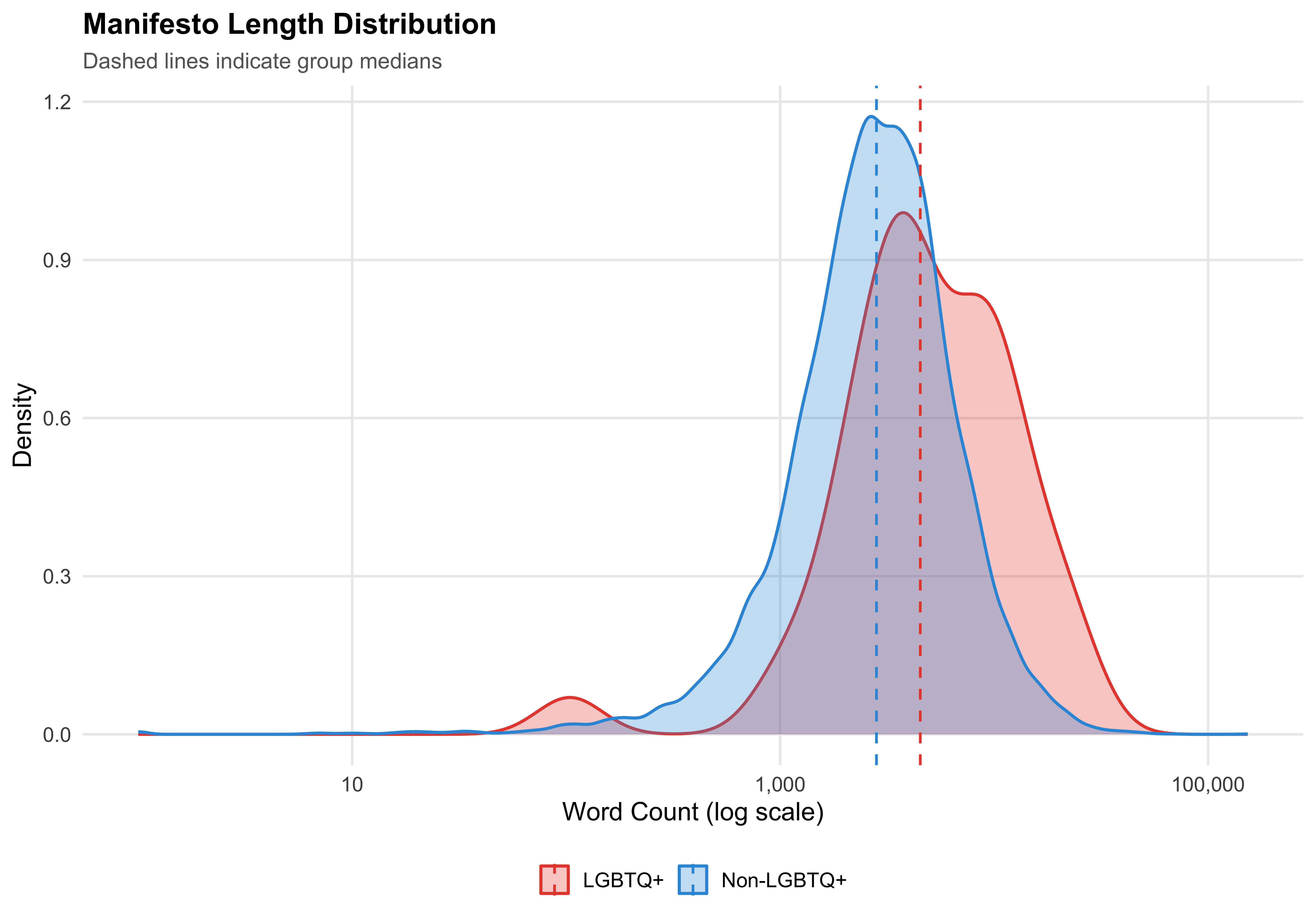
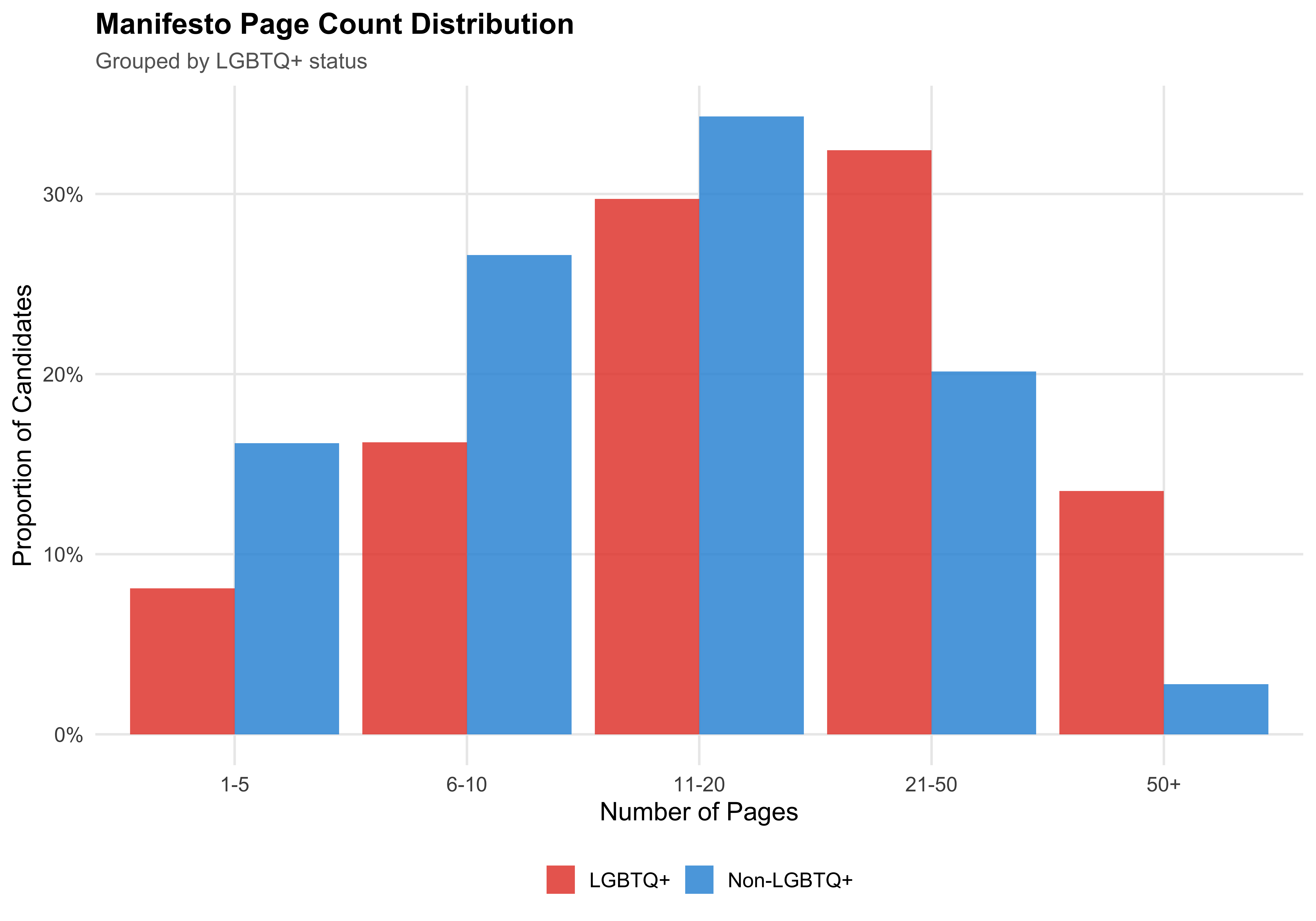
LGBTQ+ candidates write manifestos that are `r word_direction` than those of non-LGBTQ+ candidates (median `r format_n(median_words_lgbtq)` vs `r format_n(median_words_nonlgbtq)` words). The median page count is `r median_pages_lgbtq` for LGBTQ+ candidates and `r median_pages_nonlgbtq` for non-LGBTQ+ candidates.
## Word Count Distribution
```{r fig-word-count-density}
#| label: fig-word-count-density
#| fig-cap: "Distribution of Manifesto Word Counts by LGBTQ+ Status (Log Scale)"
ggplot(mayors, aes(x = manifesto_n_words, fill = lgbtq_label, color = lgbtq_label)) +
  geom_density(alpha = 0.3, linewidth = 0.8) +
  geom_vline(
    data = mayors %>% group_by(lgbtq_label) %>%
      summarise(med = median(manifesto_n_words, na.rm = TRUE), .groups = "drop"),
    aes(xintercept = med, color = lgbtq_label),
    linetype = "dashed", linewidth = 0.7
  ) +
  scale_x_log10(labels = label_comma()) +
  scale_fill_manual(values = pal_lgbtq) +
  scale_color_manual(values = pal_lgbtq) +
  labs(
    x        = "Word Count (log scale)",
    y        = "Density",
    fill     = NULL,
    color    = NULL,
    title    = "Manifesto Length Distribution",
    subtitle = "Dashed lines indicate group medians"
  )

save_figure(last_plot(), "07_word_count_density")
```
## Page Count Distribution
```{r fig-page-count-bar}
#| label: fig-page-count-bar
#| fig-cap: "Page Count Distribution by LGBTQ+ Status"
mayors %>%
  mutate(page_bin = cut(
    manifesto_n_pages,
    breaks = c(0, 5, 10, 20, 50, Inf),
    labels = c("1-5", "6-10", "11-20", "21-50", "50+"),
    right = TRUE
  )) %>%
  count(lgbtq_label, page_bin) %>%
  group_by(lgbtq_label) %>%
  mutate(pct = n / sum(n)) %>%
  ungroup() %>%
  ggplot(aes(x = page_bin, y = pct, fill = lgbtq_label)) +
  geom_col(position = "dodge", alpha = 0.85) +
  scale_y_continuous(labels = label_percent()) +
  scale_fill_manual(values = pal_lgbtq) +
  labs(
    x        = "Number of Pages",
    y        = "Proportion of Candidates",
    fill     = NULL,
    title    = "Manifesto Page Count Distribution",
    subtitle = "Grouped by LGBTQ+ status"
  )

save_figure(last_plot(), "07_page_count_dist")
```
## Word Count by Identity Category
```{r tbl-wordcount-identity}
#| label: tbl-wordcount-identity
#| tbl-cap: "Manifesto Length by LGBTQ+ Identity Category"
identity_words <- mayors %>%
  filter(lgbtq_candidate, lgbt_category != "Other LGBTQ+") %>%
  group_by(lgbt_category) %>%
  summarise(
    N              = n(),
    `Median Words` = format_n(median(manifesto_n_words, na.rm = TRUE)),
    `Mean Words`   = format_n(round(mean(manifesto_n_words, na.rm = TRUE))),
    `Median Pages` = round(median(manifesto_n_pages, na.rm = TRUE), 1),
    .groups = "drop"
  ) %>%
  rename(Category = lgbt_category) %>%
  arrange(desc(N))

# Add Non-LGBTQ+ reference row
nonlgbtq_ref <- tibble(
  Category       = "Non-LGBTQ+ (ref.)",
  N              = n_nonlgbtq,
  `Median Words` = format_n(median_words_nonlgbtq),
  `Mean Words`   = format_n(round(mean_words_nonlgbtq)),
  `Median Pages` = round(median_pages_nonlgbtq, 1)
)

bind_rows(identity_words, nonlgbtq_ref) %>%
  kable(align = c("l", "r", "r", "r", "r"))
save_table(bind_rows(identity_words, nonlgbtq_ref), "07_wordcount_identity.csv")
```
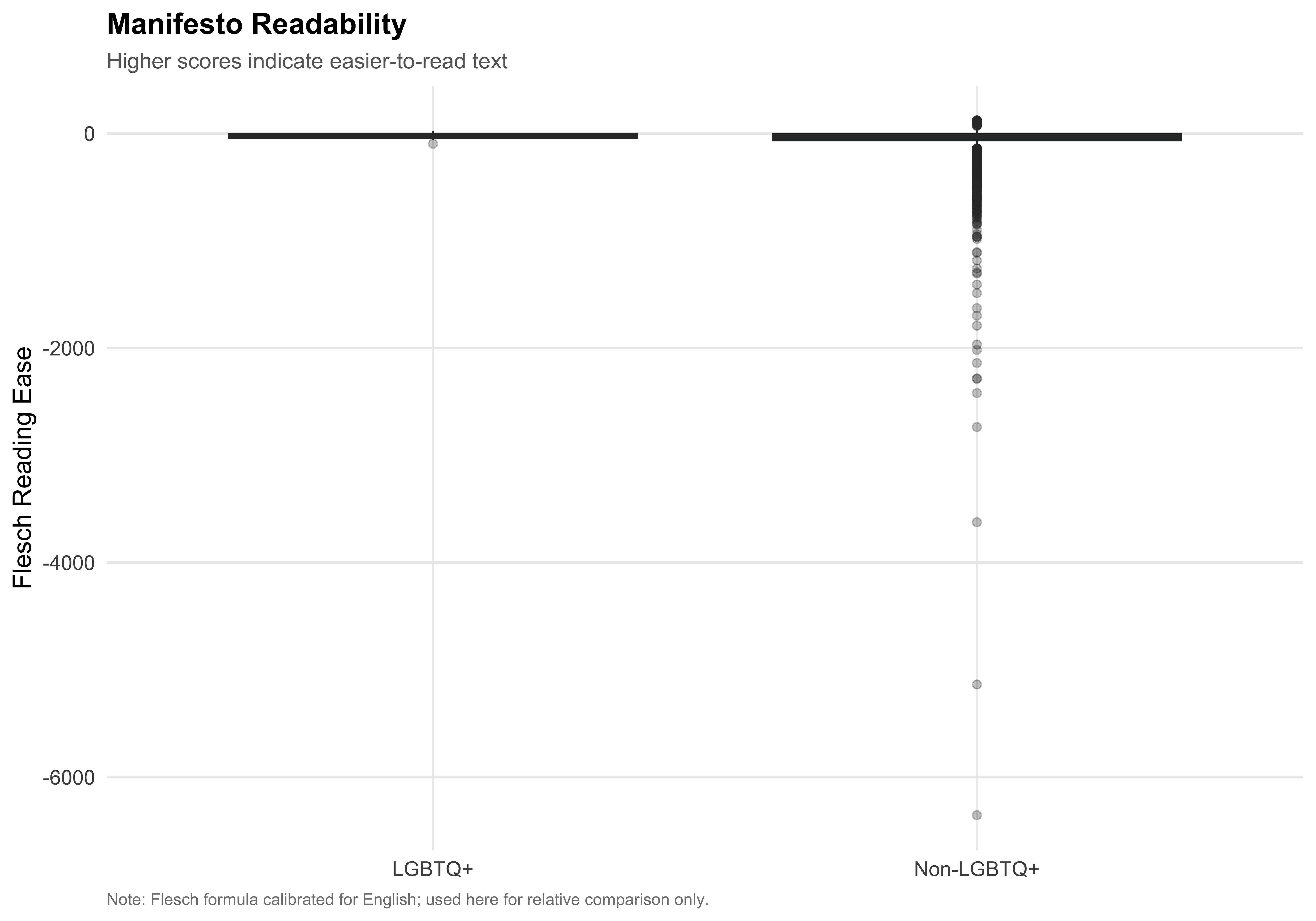
# Text Complexity
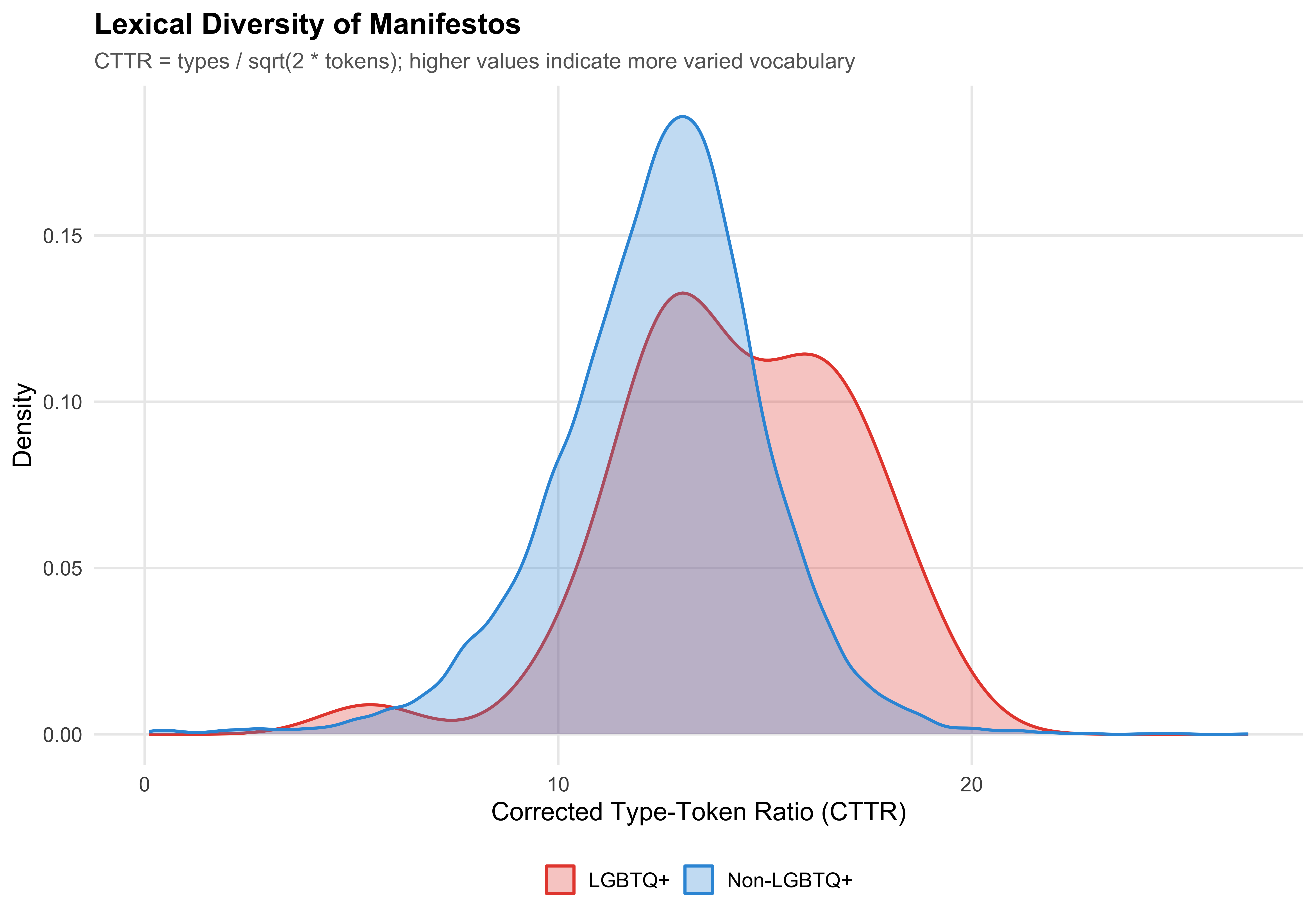
We examine two dimensions of text complexity: **readability** (how easy the text is to read) and **lexical diversity** (how varied the vocabulary is).
::: {.callout-note}
## Readability Caveat
The Flesch Reading Ease formula was developed for English. While its syllable-counting mechanics work for Portuguese text, the absolute scores are not directly interpretable as US grade levels. We use these scores only for *relative* comparisons between groups, not for absolute readability claims.
:::
```{r manifesto-text-complexity}
# Build quanteda corpus
corp <- corpus(mayors, text_field = "manifesto_text",
               docid_field = "candidate_id")

# Readability (Flesch)
readability <- textstat_readability(corp, measure = "Flesch") %>%
  rename(candidate_id = document, flesch = Flesch) %>%
  mutate(candidate_id = as.numeric(candidate_id))

# Lexical diversity (CTTR — Corrected Type-Token Ratio)
# Note: MATTR crashes on quanteda.textstats 0.97.2 (window reset bug).
# CTTR = types / sqrt(2 * tokens), which also corrects for document length.
toks_lexdiv <- tokens(corp, remove_punct = TRUE, remove_numbers = TRUE)
lexdiv <- textstat_lexdiv(toks_lexdiv, measure = "CTTR") %>%
  rename(candidate_id = document, cttr = CTTR) %>%
  mutate(candidate_id = as.numeric(candidate_id))

# Join back to mayors
mayors <- mayors %>%
  left_join(readability, by = "candidate_id") %>%
  left_join(lexdiv, by = "candidate_id")
```
## Readability Comparison
```{r fig-readability-comparison}
#| label: fig-readability-comparison
#| fig-cap: "Flesch Reading Ease Score by LGBTQ+ Status"
ggplot(mayors, aes(x = lgbtq_label, y = flesch, fill = lgbtq_label)) +
  geom_boxplot(alpha = 0.7, outlier.alpha = 0.3) +
  scale_fill_manual(values = pal_lgbtq) +
  labs(
    x        = NULL,
    y        = "Flesch Reading Ease",
    fill     = NULL,
    title    = "Manifesto Readability",
    subtitle = "Higher scores indicate easier-to-read text",
    caption  = "Note: Flesch formula calibrated for English; used here for relative comparison only."
  ) +
  guides(fill = "none")

save_figure(last_plot(), "07_readability_comparison")
```
## Lexical Diversity
```{r fig-lexdiv-comparison}
#| label: fig-lexdiv-comparison
#| fig-cap: "Lexical Diversity (CTTR) by LGBTQ+ Status"
ggplot(mayors, aes(x = cttr, fill = lgbtq_label, color = lgbtq_label)) +
  geom_density(alpha = 0.3, linewidth = 0.8) +
  scale_fill_manual(values = pal_lgbtq) +
  scale_color_manual(values = pal_lgbtq) +
  labs(
    x        = "Corrected Type-Token Ratio (CTTR)",
    y        = "Density",
    fill     = NULL,
    color    = NULL,
    title    = "Lexical Diversity of Manifestos",
    subtitle = "CTTR = types / sqrt(2 * tokens); higher values indicate more varied vocabulary"
  )

save_figure(last_plot(), "07_lexdiv_comparison")
```
## Complexity Summary
```{r tbl-text-complexity}
#| label: tbl-text-complexity
#| tbl-cap: "Text Complexity Summary by LGBTQ+ Status"
# Wilcoxon tests
flesch_test <- wilcox.test(flesch ~ lgbtq_label, data = mayors)
cttr_test   <- wilcox.test(cttr ~ lgbtq_label, data = mayors)

format_p <- function(p) {
  if (p < 0.001) "< 0.001" else sprintf("%.3f", p)
}

complexity_summary <- mayors %>%
  group_by(lgbtq_label) %>%
  summarise(
    N               = n(),
    `Median Flesch`  = round(median(flesch, na.rm = TRUE), 1),
    `Mean Flesch`    = round(mean(flesch, na.rm = TRUE), 1),
    `Median CTTR`    = round(median(cttr, na.rm = TRUE), 3),
    `Mean CTTR`      = round(mean(cttr, na.rm = TRUE), 3),
    .groups = "drop"
  ) %>%
  rename(Group = lgbtq_label)

complexity_summary %>% kable(align = c("l", "r", "r", "r", "r", "r"))
save_table(complexity_summary, "07_text_complexity.csv")
```
Wilcoxon rank-sum test: Flesch p = `r format_p(flesch_test$p.value)`; CTTR p = `r format_p(cttr_test$p.value)`.
# Word Frequency and Keyness
```{r manifesto-nlp-pipeline}
# --- Build the NLP pipeline (shared across sections 4-6) ---

# Portuguese stopwords: combine two sources for broad coverage
pt_stopwords <- unique(c(
  stopwords("pt", source = "snowball"),
  stopwords("pt", source = "stopwords-iso")
))

# Domain-specific stopwords common in Brazilian political manifestos
manifesto_stopwords <- c(
  "município", "municipio", "cidade", "prefeito", "prefeita",
  "vice", "candidato", "candidata", "governo", "plano",
  "proposta", "propostas", "gestão", "gestao", "administração",
  "administracao", "público", "publico", "pública", "publica",
  "municipal", "prefeitura", "câmara", "camara", "vereador",
  "secretaria", "artigo", "lei", "parágrafo", "inciso",
  "nº", "art", "cf", "cpf", "cnpj", "ainda", "além", "cada",
  "forma", "bem", "toda", "todo", "todos", "todas", "será",
  "deve", "deverá", "podem", "podem", "sendo", "através",
  "assim", "sobre", "entre", "onde", "acordo", "partir"
)

all_stopwords <- unique(c(pt_stopwords, manifesto_stopwords))

# Tokenize
toks <- tokens(corp, remove_punct = TRUE, remove_numbers = TRUE,
               remove_symbols = TRUE) %>%
  tokens_tolower() %>%
  tokens_remove(pattern = all_stopwords) %>%
  tokens_remove(pattern = "^.{1,2}$", valuetype = "regex")

# Stemmed version for frequency and STM
toks_stem <- tokens_wordstem(toks, language = "portuguese")

# DFMs
dfm_raw  <- dfm(toks)        # unstemmed (for dictionary lookup)
dfm_stem <- dfm(toks_stem)   # stemmed

# Trimmed version for keyness and STM
# Convert count threshold to proportion (compatible with all quanteda versions)
dfm_trimmed <- dfm_stem %>%
  dfm_trim(min_docfreq = 10 / ndoc(dfm_stem), max_docfreq = 0.95,
           docfreq_type = "prop")
```
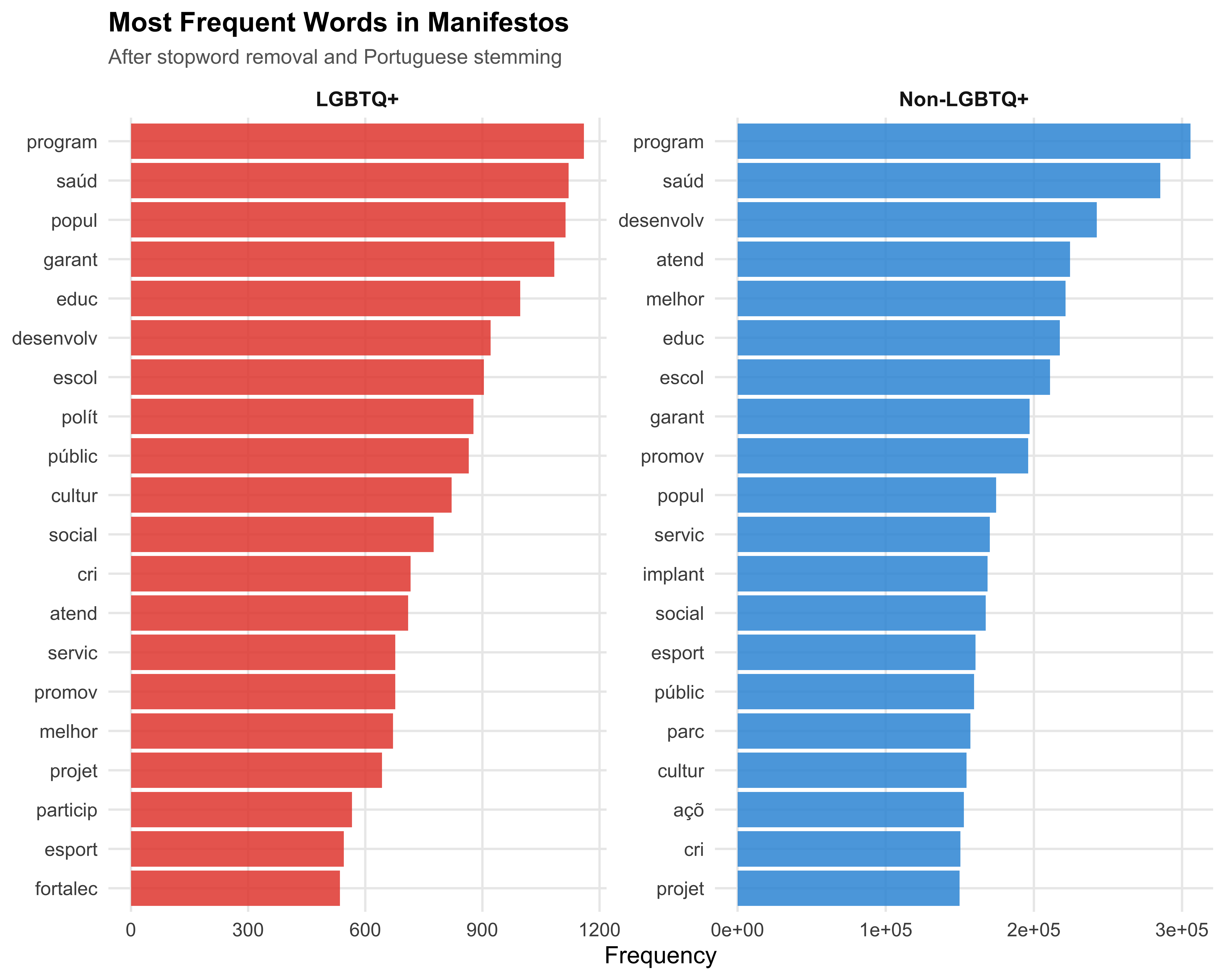
## Top Words by Group
```{r fig-top-words-group}
#| label: fig-top-words-group
#| fig-cap: "Top 20 Most Frequent Stemmed Words by LGBTQ+ Status"
#| fig-height: 8
# Group DFM by LGBTQ+ label
dfm_grouped <- dfm_group(dfm_stem, groups = lgbtq_label)

# Get top words per group
top_words <- textstat_frequency(dfm_stem, n = 20, groups = lgbtq_label) %>%
  mutate(group = factor(group, levels = c("LGBTQ+", "Non-LGBTQ+")))

ggplot(top_words, aes(x = reorder_within(feature, frequency, group),
                      y = frequency, fill = group)) +
  geom_col(alpha = 0.85, show.legend = FALSE) +
  scale_x_reordered() +
  scale_fill_manual(values = pal_lgbtq) +
  coord_flip() +
  facet_wrap(~ group, scales = "free") +
  labs(
    x     = NULL,
    y     = "Frequency",
    title = "Most Frequent Words in Manifestos",
    subtitle = "After stopword removal and Portuguese stemming"
  )

save_figure(last_plot(), "07_top_words_group", height = 8)
```
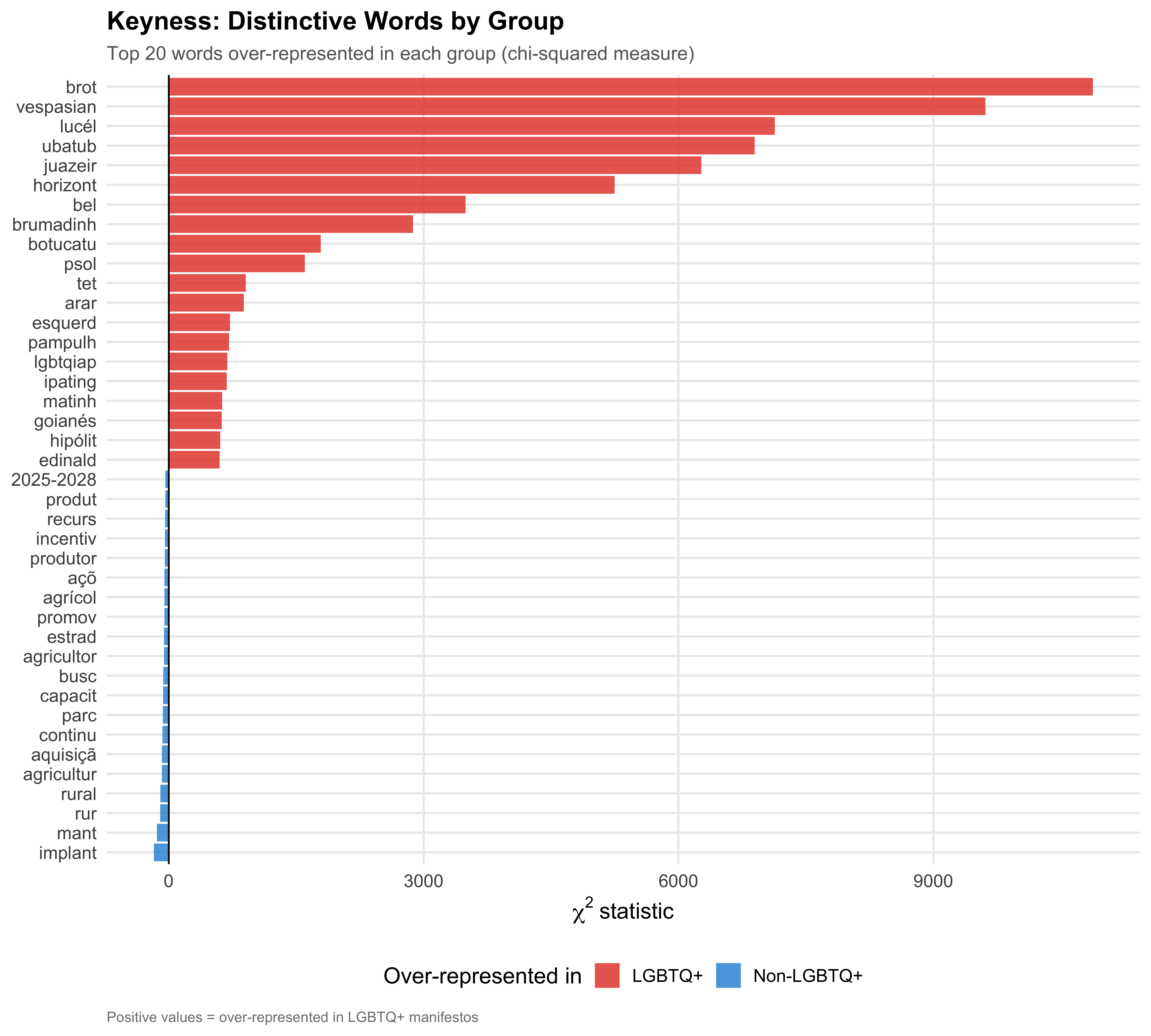
## Keyness Analysis
Keyness statistics identify words that appear *disproportionately* in one group relative to the other. We use the chi-squared measure, with LGBTQ+ manifestos as the target group.
```{r fig-keyness-plot}
#| label: fig-keyness-plot
#| fig-cap: "Statistical Keyness: Words Over-Represented in LGBTQ+ vs Non-LGBTQ+ Manifestos"
#| fig-height: 9
# Group and compute keyness
dfm_key <- dfm_group(dfm_trimmed, groups = lgbtq_label)
keyness <- textstat_keyness(dfm_key, target = "LGBTQ+", measure = "chi2")

# Top 20 in each direction
top_pos <- keyness %>% slice_max(chi2, n = 20)
top_neg <- keyness %>% slice_min(chi2, n = 20)
key_plot_data <- bind_rows(top_pos, top_neg) %>%
  mutate(
    direction = if_else(chi2 > 0, "LGBTQ+", "Non-LGBTQ+"),
    feature   = reorder(feature, chi2)
  )

ggplot(key_plot_data, aes(x = chi2, y = feature, fill = direction)) +
  geom_col(alpha = 0.85) +
  geom_vline(xintercept = 0, linewidth = 0.5) +
  scale_fill_manual(values = pal_lgbtq) +
  labs(
    x        = expression(chi^2 ~ "statistic"),
    y        = NULL,
    fill     = "Over-represented in",
    title    = "Keyness: Distinctive Words by Group",
    subtitle = "Top 20 words over-represented in each group (chi-squared measure)",
    caption  = "Positive values = over-represented in LGBTQ+ manifestos"
  )

save_figure(last_plot(), "07_keyness_chi2", height = 9)
```
::: {.callout-note}
## Interpreting Keyness
A high positive chi-squared value means the word is overrepresented in LGBTQ+ manifestos relative to their size; a high negative value means it is overrepresented in non-LGBTQ+ manifestos. With only `r format_n(n_lgbtq)` LGBTQ+ documents, individual keyness scores should be treated as exploratory indicators rather than definitive findings.
:::
# Policy Dictionary Analysis
We define a custom Portuguese-language policy dictionary with 10 domains covering the main areas of Brazilian municipal governance. Each manifesto's salience profile is the proportion of its (classified) words falling in each domain.
```{r manifesto-policy-dictionary}
policy_dict <- dictionary(list(
  education = c(
    "educação", "educacao", "escola*", "escolar*", "ensino", "professor*",
    "aluno*", "estudant*", "creche*", "infantil", "fundamental",
    "pedagóg*", "pedagogic*", "aprendizagem", "alfabetização",
    "alfabetizacao", "universidade", "faculdade", "merenda",
    "biblioteca*", "letiv*", "curricul*"
  ),
  health = c(
    "saúde", "saude", "hospital*", "ubs", "upa", "médic*", "medic*",
    "enferm*", "vacina*", "atendimento", "emergência", "emergencia",
    "ambulância", "ambulancia", "sus", "farmácia", "farmacia",
    "odontológ*", "odontolog*", "mental", "psicológ*", "psicolog*",
    "terapêut*", "terapia", "maternidade"
  ),
  security = c(
    "segurança", "seguranca", "polícia*", "policia*", "guarda",
    "vigilância", "vigilancia", "câmera*", "camera*", "iluminação",
    "iluminacao", "violência", "violencia", "crime*", "criminal*",
    "tráfico", "trafico", "droga*", "patrulha*", "ronda*"
  ),
  economy = c(
    "emprego*", "trabalho", "econom*", "renda", "empreend*",
    "empresa*", "comércio", "comercio", "indústria", "industria",
    "turismo", "agricultur*", "cooperativ*", "microcrédito",
    "microcredito", "capacitação", "capacitacao", "desenvolviment*",
    "investiment*", "fiscal", "orçament*", "orcament*"
  ),
  social_policy = c(
    "assistência social", "assistencia social", "vulnerab*",
    "pobreza", "benefício", "beneficio", "cras", "creas",
    "idoso*", "criança*", "crianca*", "adolescente*", "juventude",
    "igualdade", "inclusão", "inclusao", "acessibilidade",
    "deficien*", "habitação", "habitacao", "moradia"
  ),
  environment = c(
    "ambiental*", "sustentab*", "ecológ*", "ecolog*",
    "reciclagem", "resíduo*", "residuo*", "lixo", "saneamento",
    "esgoto", "desmatamento", "reflorestamento",
    "poluição", "poluicao", "clima*", "energia solar",
    "preservação", "preservacao", "parque*"
  ),
  infrastructure = c(
    "infraestrutura", "pavimentação", "pavimentacao", "asfalto",
    "transporte", "ônibus", "onibus", "mobilidade", "trânsito",
    "transito", "estrada*", "ponte*", "construção",
    "construcao", "urbaniz*", "drenagem", "calçada*", "calcada*",
    "ciclovia*"
  ),
  lgbtq_rights = c(
    "lgbt*", "diversidade sexual", "orientação sexual",
    "orientacao sexual", "identidade de gênero", "identidade de genero",
    "homofob*", "transfob*", "travesti*", "transgêner*", "transgenero*",
    "lésbica*", "lesbica*", "bisexual*", "queer",
    "nome social"
  ),
  culture = c(
    "cultur*", "arte*", "artístic*", "artistic*", "museu*",
    "teatro*", "cinema", "festival*", "patrimônio", "patrimonio",
    "esporte*", "esportiv*", "lazer", "recreação", "recreacao"
  ),
  transparency = c(
    "transparência", "transparencia", "participação popular",
    "participacao popular", "conselho*", "audiência pública",
    "audiencia publica", "orçamento participativo",
    "orcamento participativo", "fiscalização", "fiscalizacao",
    "prestação de contas", "prestacao de contas",
    "ouvidoria", "dados abertos"
  )
))
```
```{r manifesto-dict-apply}
# Apply dictionary to unstemmed tokens (dictionary entries use their own glob patterns)
dfm_dict <- dfm_lookup(dfm_raw, dictionary = policy_dict)

# Convert to proportions (salience = share of classified words per domain)
dfm_dict_prop <- dfm_weight(dfm_dict, scheme = "prop")

# Convert to tidy data frame
dict_results <- convert(dfm_dict_prop, to = "data.frame") %>%
  pivot_longer(-doc_id, names_to = "policy_domain", values_to = "salience") %>%
  mutate(doc_id = as.numeric(doc_id)) %>%
  left_join(
    mayors %>% select(candidate_id, lgbtq_candidate, lgbtq_label,
                      lgbt_category, ideology_category, region, state_abbrev),
    by = c("doc_id" = "candidate_id")
  )

# Clean domain labels for display
domain_labels <- c(
  education      = "Education",
  health         = "Health",
  security       = "Security",
  economy        = "Economy",
  social_policy  = "Social Policy",
  environment    = "Environment",
  infrastructure = "Infrastructure",
  lgbtq_rights   = "LGBTQ+ Rights",
  culture        = "Culture",
  transparency   = "Transparency"
)

dict_results <- dict_results %>%
  mutate(domain_label = domain_labels[policy_domain])
```
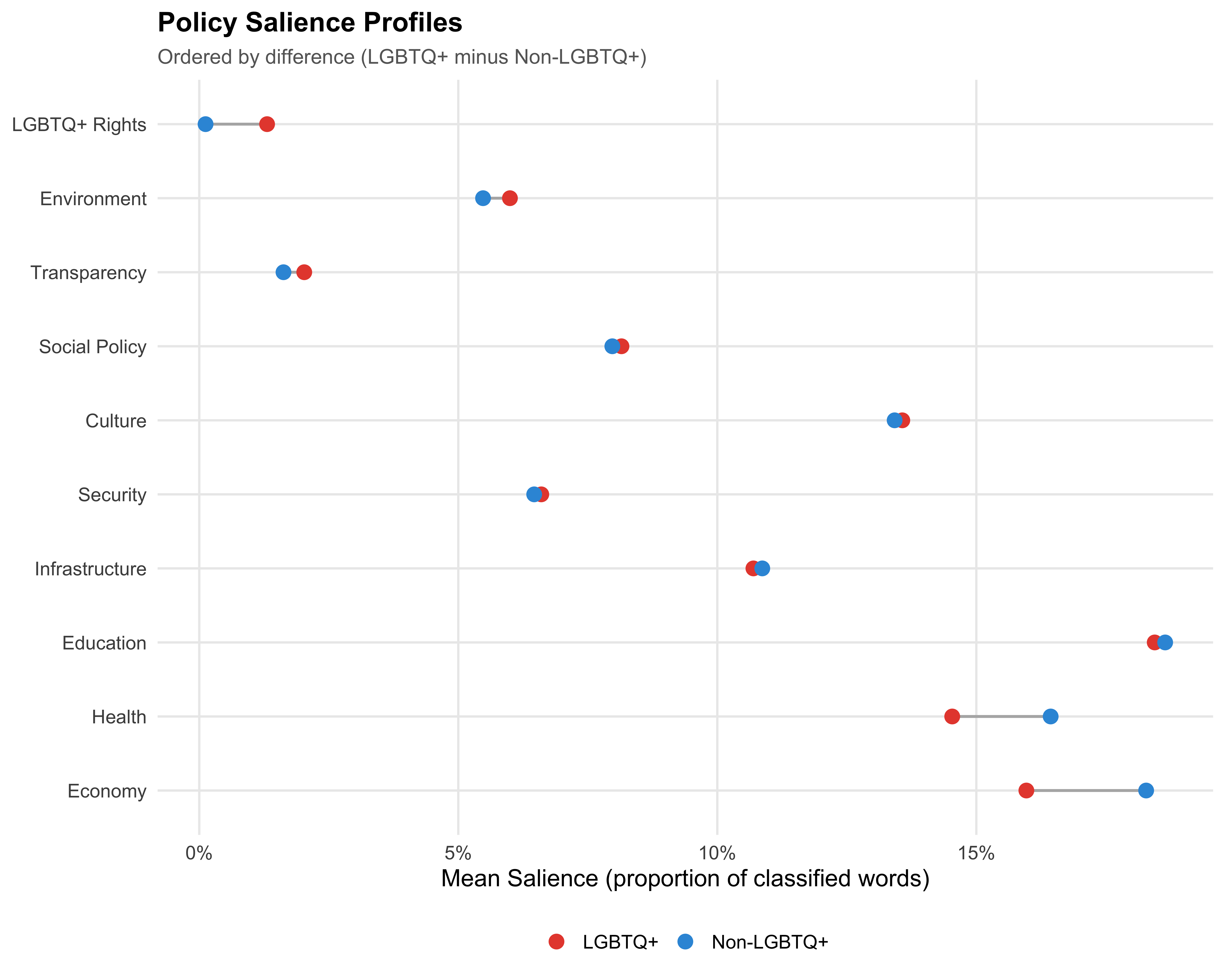
## Salience Comparison
```{r tbl-salience-comparison}
#| label: tbl-salience-comparison
#| tbl-cap: "Mean Policy Salience by Domain and LGBTQ+ Status"
salience_by_group <- dict_results %>%
  group_by(domain_label, lgbtq_label) %>%
  summarise(mean_sal = mean(salience, na.rm = TRUE), .groups = "drop") %>%
  pivot_wider(names_from = lgbtq_label, values_from = mean_sal) %>%
  mutate(Difference = `LGBTQ+` - `Non-LGBTQ+`)

# Wilcoxon tests per domain
wilcox_p <- dict_results %>%
  group_by(domain_label) %>%
  summarise(
    p_value = wilcox.test(salience ~ lgbtq_label)$p.value,
    .groups = "drop"
  ) %>%
  mutate(p_fmt = sapply(p_value, format_p))

salience_table <- salience_by_group %>%
  left_join(wilcox_p %>% select(domain_label, p_fmt), by = "domain_label") %>%
  arrange(desc(abs(Difference))) %>%
  mutate(
    `LGBTQ+`      = format_pct(`LGBTQ+`),
    `Non-LGBTQ+`  = format_pct(`Non-LGBTQ+`),
    Difference     = sprintf("%+.1f pp", Difference * 100)
  ) %>%
  rename(Domain = domain_label, `Wilcoxon p` = p_fmt)

salience_table %>% kable(align = c("l", "r", "r", "r", "r"))
save_table(salience_table, "07_salience_comparison.csv")
```
## Salience Profile
```{r fig-salience-profile}
#| label: fig-salience-profile
#| fig-cap: "Policy Salience Profiles: LGBTQ+ vs Non-LGBTQ+ Candidates"
#| fig-height: 8
salience_plot_data <- dict_results %>%
  group_by(domain_label, lgbtq_label) %>%
  summarise(mean_sal = mean(salience, na.rm = TRUE), .groups = "drop")

# Order domains by difference
domain_order <- salience_plot_data %>%
  pivot_wider(names_from = lgbtq_label, values_from = mean_sal) %>%
  mutate(diff = `LGBTQ+` - `Non-LGBTQ+`) %>%
  arrange(diff) %>%
  pull(domain_label)

salience_plot_data <- salience_plot_data %>%
  mutate(domain_label = factor(domain_label, levels = domain_order))

ggplot(salience_plot_data, aes(x = mean_sal, y = domain_label,
                               color = lgbtq_label)) +
  geom_line(aes(group = domain_label), color = "grey70", linewidth = 0.8) +
  geom_point(size = 3.5) +
  scale_x_continuous(labels = label_percent()) +
  scale_color_manual(values = pal_lgbtq) +
  labs(
    x        = "Mean Salience (proportion of classified words)",
    y        = NULL,
    color    = NULL,
    title    = "Policy Salience Profiles",
    subtitle = "Ordered by difference (LGBTQ+ minus Non-LGBTQ+)"
  )

save_figure(last_plot(), "07_salience_profile", height = 8)
```
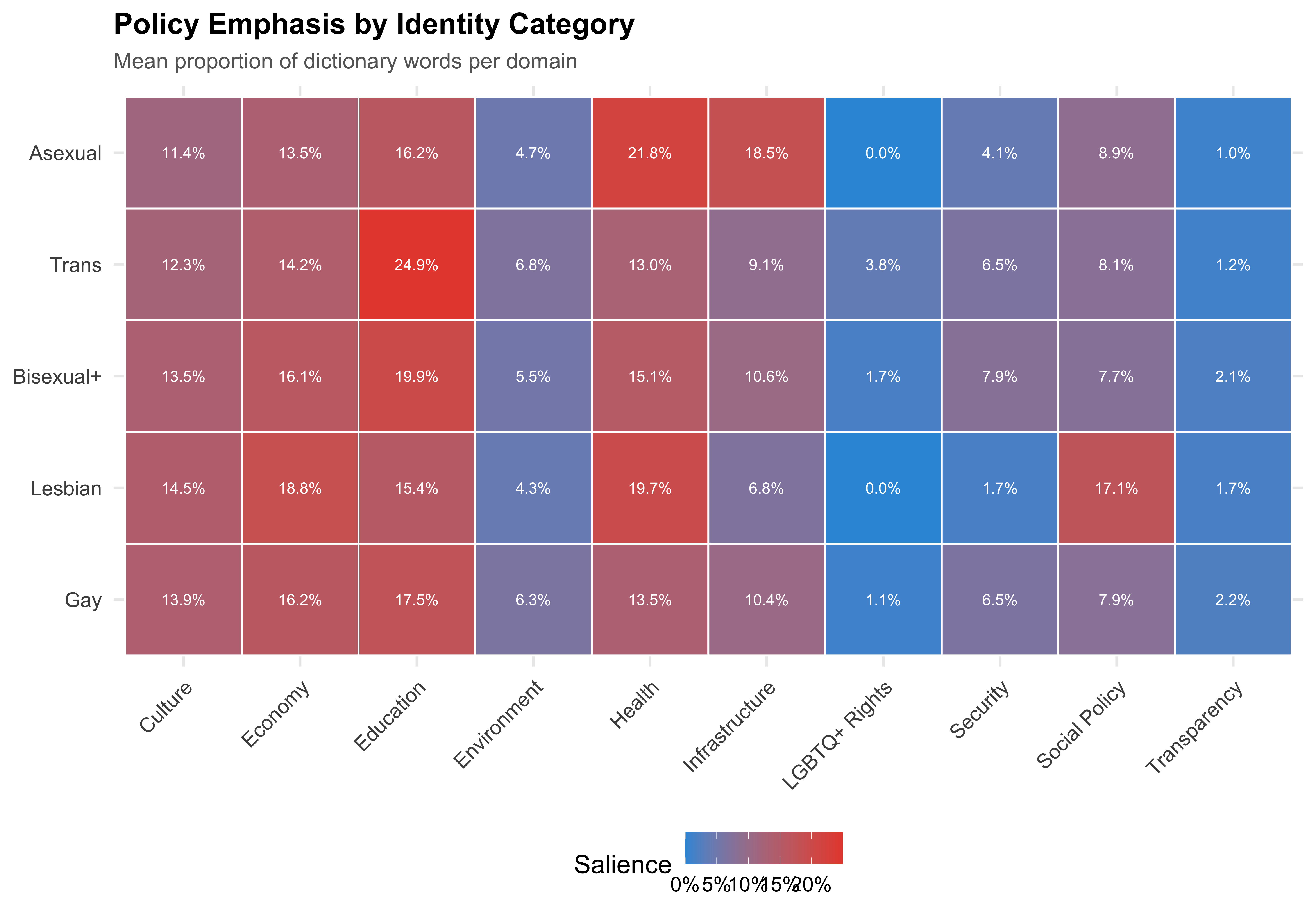
## Salience by Identity Category
```{r fig-salience-identity}
#| label: fig-salience-identity
#| fig-cap: "Policy Salience Heatmap by LGBTQ+ Identity Category"
#| fig-height: 7
identity_salience <- dict_results %>%
  filter(lgbtq_candidate, !is.na(lgbt_category),
         lgbt_category != "Other LGBTQ+") %>%
  group_by(lgbt_category, domain_label) %>%
  summarise(mean_sal = mean(salience, na.rm = TRUE), .groups = "drop")

ggplot(identity_salience, aes(x = domain_label, y = lgbt_category,
                               fill = mean_sal)) +
  geom_tile(color = "white", linewidth = 0.5) +
  geom_text(aes(label = sprintf("%.1f%%", mean_sal * 100)),
            size = 3, color = "white") +
  scale_fill_gradient(low = "#3498DB", high = "#E74C3C",
                      labels = label_percent()) +
  labs(
    x     = NULL,
    y     = NULL,
    fill  = "Salience",
    title = "Policy Emphasis by Identity Category",
    subtitle = "Mean proportion of dictionary words per domain"
  ) +
  theme(axis.text.x = element_text(angle = 45, hjust = 1))

save_figure(last_plot(), "07_salience_identity_heatmap")
```
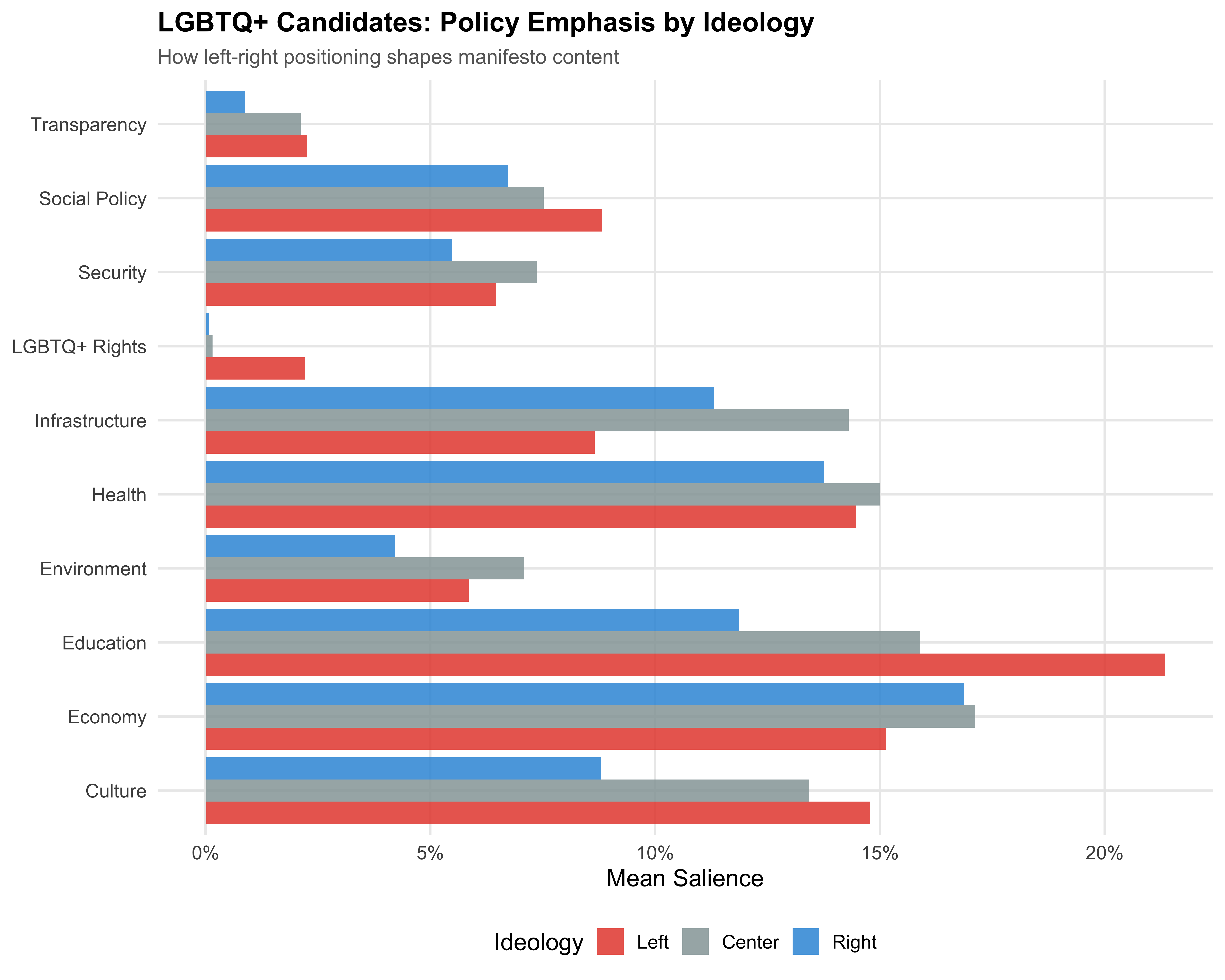
## Salience by Ideology
```{r fig-salience-ideology}
#| label: fig-salience-ideology
#| fig-cap: "Policy Salience by Ideology Among LGBTQ+ Candidates"
#| fig-height: 8
ideology_salience <- dict_results %>%
  filter(lgbtq_candidate, !is.na(ideology_category)) %>%
  group_by(ideology_category, domain_label) %>%
  summarise(mean_sal = mean(salience, na.rm = TRUE), .groups = "drop")

ggplot(ideology_salience, aes(x = mean_sal, y = domain_label,
                               fill = ideology_category)) +
  geom_col(position = "dodge", alpha = 0.85) +
  scale_x_continuous(labels = label_percent()) +
  scale_fill_manual(values = pal_ideology) +
  labs(
    x        = "Mean Salience",
    y        = NULL,
    fill     = "Ideology",
    title    = "LGBTQ+ Candidates: Policy Emphasis by Ideology",
    subtitle = "How left-right positioning shapes manifesto content"
  )

save_figure(last_plot(), "07_salience_ideology", height = 8)
```
::: {.callout-note}
## Dictionary Limitations
Dictionary methods capture only *explicit* mentions of policy keywords. A candidate may address a topic using indirect language, metaphors, or euphemisms that the dictionary does not capture. Additionally, some words belong to multiple domains (e.g., "comunidade" could be social policy or infrastructure). These results indicate *explicit policy emphasis*, not comprehensive measures of issue attention.
:::
<!-- HIDDEN: Structural Topic Model (temporarily removed from website output)
# Structural Topic Model
The Structural Topic Model (STM) identifies latent topics in the corpus and estimates whether LGBTQ+ status predicts different topic emphasis, controlling for ideology and region.
```{r stm-prepare}
#| output: false
# Prepare DFM for STM: remove empty documents after trimming
dfm_stm <- dfm_subset(dfm_trimmed, ntoken(dfm_trimmed) > 0)
# Align metadata with DFM documents
stm_meta <- mayors[match(docnames(dfm_stm), as.character(mayors$candidate_id)), ] %>%
mutate(
lgbtq = as.integer(lgbtq_candidate),
ideology_num = case_when(
ideology_category == "Left" ~ -1,
ideology_category == "Center" ~ 0,
ideology_category == "Right" ~ 1,
TRUE ~ NA_real_
)
)
# Drop rows with NA ideology or region (STM cannot handle NAs in prevalence covariates)
complete_idx <- !is.na(stm_meta$ideology_num) & !is.na(stm_meta$region)
dfm_stm <- dfm_subset(dfm_stm, complete_idx)
stm_meta <- stm_meta[complete_idx, ]
# Convert to STM format
stm_converted <- convert(dfm_stm, to = "stm")
```
## Selecting the Number of Topics
```{r stm-searchk}
#| label: stm-searchk
#| cache: true
#| output: false
set.seed(2024)
k_search <- searchK(
documents = stm_converted$documents,
vocab = stm_converted$vocab,
K = c(10, 15, 20, 25),
prevalence = ~ lgbtq + ideology_num + region,
data = stm_meta,
init.type = "Spectral",
cores = 1
)
```
```{r fig-stm-searchk}
#| label: fig-stm-searchk
#| fig-cap: "STM Model Selection Diagnostics Across K Values"
#| fig-height: 8
# Extract searchK results into a data frame
sk_results <- data.frame(
K = unlist(k_search$results$K),
exclus = unlist(k_search$results$exclus),
semcoh = unlist(k_search$results$semcoh),
heldout = unlist(k_search$results$heldout),
residual = unlist(k_search$results$residual)
)
p1 <- ggplot(sk_results, aes(x = K, y = semcoh)) +
geom_line(linewidth = 1) + geom_point(size = 3) +
labs(x = "K", y = "Semantic Coherence", title = "Semantic Coherence")
p2 <- ggplot(sk_results, aes(x = K, y = exclus)) +
geom_line(linewidth = 1) + geom_point(size = 3) +
labs(x = "K", y = "Exclusivity", title = "Exclusivity")
p3 <- ggplot(sk_results, aes(x = K, y = heldout)) +
geom_line(linewidth = 1) + geom_point(size = 3) +
labs(x = "K", y = "Held-Out Likelihood", title = "Held-Out Likelihood")
p4 <- ggplot(sk_results, aes(x = K, y = residual)) +
geom_line(linewidth = 1) + geom_point(size = 3) +
labs(x = "K", y = "Residuals", title = "Residual Dispersion")
(p1 + p2) / (p3 + p4) +
plot_annotation(
title = "STM Model Selection",
subtitle = "Diagnostics across different numbers of topics (K)"
)
save_figure(last_plot(), "07_stm_searchk", height = 8)
```
::: {.callout-note}
## Selecting K
We evaluate models with K = 10, 15, 20, and 25 topics using four diagnostics: semantic coherence (do top words co-occur?), exclusivity (are top words unique to topics?), held-out likelihood (predictive fit), and residual dispersion. We select K = 15 as a balance between coherence and exclusivity, favoring interpretability for a descriptive analysis.
:::
## Fit Selected Model
```{r stm-fit}
#| cache: true
K_selected <- 15
set.seed(2024)
stm_fit <- stm(
documents = stm_converted$documents,
vocab = stm_converted$vocab,
K = K_selected,
prevalence = ~ lgbtq + ideology_num + region,
data = stm_meta,
init.type = "Spectral",
max.em.its = 150,
verbose = FALSE
)
```
## Topic Labels
```{r tbl-stm-topics}
#| label: tbl-stm-topics
#| tbl-cap: "STM Topics: Interpretive Labels, Top Words, and Descriptions"
topic_labels <- labelTopics(stm_fit, n = 7)
# Interpretive labels based on top FREX and probability words
topic_names <- c(
"Public Incentives & Guarantees",
"Women's Centres & Education",
"Rural Development & Traditions",
"OCR Artefacts / Formatting",
"Social Assistance & Services",
"Party Coalitions & Governance",
"Diversity, Rights & Inclusion",
"Sustainable Development",
"Infrastructure & Road Works",
"Fiscal Criticism & Budgets",
"Health & Social Service Expansion",
"Urban Infrastructure & Transport",
"Transparency & Public Admin",
"Tourism, Agriculture & Culture",
"Governance Principles & Policy"
)
topic_descriptions <- c(
"Tax incentives, public guarantees, and economic development programmes",
"Community centres for women, educational programmes, and gender-focused services (includes city-specific OCR terms)",
"Rural zones, traditional cultural events (e.g., vaquejada), agricultural slaughterhouses, and school uniforms",
"Residual topic capturing formatting artefacts from PDF extraction (stop-words, punctuation with control characters)",
"Social assistance networks, socio-educational programmes, and public service delivery",
"Electoral coalitions, party alliances (PSD, MDB, PDT, PSB), and coalition governance language",
"Racial equality, anti-racism, indigenous rights, LGBTQI+ inclusion, and left-party (PSOL) social justice framing",
"Well-being, sustainability, citizen engagement, and long-term development challenges",
"Road construction materials (gravel, limestone), truck logistics, and rural infrastructure (Paraná-area terms)",
"Budgetary criticism, fiscal figures (millions/billions), and opposition-style problem framing",
"Expansion and strengthening of multi-professional health teams and social assistance networks",
"Urban projects: neighbourhoods, overpasses, airports, waterfront/nautical facilities, and road networks",
"Auditing, evaluation reports, accountability criteria, and public resource management",
"Tourism promotion, agricultural incentives, environmental preservation, and cultural events",
"Legal principles, policy alignment across government spheres, and normative governance language"
)
topic_table <- tibble(
Topic = 1:K_selected,
Label = topic_names,
Description = topic_descriptions,
`Top FREX Words` = apply(topic_labels$frex, 1, paste, collapse = ", "),
`Top Prob. Words` = apply(topic_labels$prob, 1, paste, collapse = ", ")
)
topic_table %>%
select(Topic, Label, Description, `Top FREX Words`) %>%
kable(align = c("r", "l", "l", "l"))
save_table(topic_table, "07_stm_topic_labels.csv")
```
::: {.callout-note}
## Reading the Topic Labels
Labels were assigned by the authors based on the highest-probability and highest-FREX (frequent and exclusive) Portuguese stems for each topic. **Topic 4** is a residual topic capturing OCR formatting artefacts from PDF extraction --- it should be disregarded in substantive interpretation. **Topic 7** ("Diversity, Rights & Inclusion") is the topic most directly related to LGBTQ+ and minority-rights discourse.
:::
## Topic Proportions
```{r fig-stm-proportions}
#| label: fig-stm-proportions
#| fig-cap: "Expected Topic Proportions Across All Manifestos"
#| fig-height: 8
topic_props <- tibble(
Topic = 1:K_selected,
Label = paste0(1:K_selected, ". ", topic_names),
Proportion = colMeans(stm_fit$theta)
)
ggplot(topic_props, aes(x = reorder(Label, Proportion), y = Proportion)) +
geom_col(fill = "#3498DB", alpha = 0.8) +
coord_flip() +
scale_y_continuous(labels = label_percent()) +
labs(
x = NULL,
y = "Expected Proportion",
title = "Overall Topic Prevalence",
subtitle = paste0("STM with K = ", K_selected, " topics")
) +
theme(axis.text.y = element_text(size = 9))
save_figure(last_plot(), "07_stm_proportions", height = 8)
```
## LGBTQ+ Effect on Topic Prevalence
```{r stm-effect}
#| output: false
stm_effect <- estimateEffect(
formula = 1:K_selected ~ lgbtq + ideology_num + region,
stmobj = stm_fit,
metadata = stm_meta,
uncertainty = "Global"
)
```
```{r tbl-stm-lgbtq-effect}
#| label: tbl-stm-lgbtq-effect
#| tbl-cap: "Effect of LGBTQ+ Status on Topic Prevalence"
# Extract LGBTQ+ coefficient for each topic
effect_summary <- map_dfr(1:K_selected, function(k) {
s <- summary(stm_effect, topics = k)
coef_table <- s$tables[[1]]
lgbtq_row <- coef_table["lgbtq", ]
tibble(
Topic = k,
Label = topic_names[k],
Estimate = lgbtq_row["Estimate"],
SE = lgbtq_row["Std. Error"],
p_value = lgbtq_row["Pr(>|t|)"]
)
}) %>%
arrange(desc(abs(Estimate)))
effect_display <- effect_summary %>%
mutate(
Estimate = sprintf("%+.4f", Estimate),
SE = sprintf("%.4f", SE),
`p-value` = sapply(p_value, format_p)
) %>%
select(Topic, Label, Estimate, SE, `p-value`)
effect_display %>% kable(align = c("r", "l", "r", "r", "r"))
save_table(effect_display, "07_stm_lgbtq_effect.csv")
```
```{r fig-stm-lgbtq-effect}
#| label: fig-stm-lgbtq-effect
#| fig-cap: "LGBTQ+ Effect on Topic Prevalence (Coefficient Plot)"
#| fig-height: 8
effect_plot_data <- effect_summary %>%
mutate(
Topic_Label = paste0(Topic, ". ", Label),
direction = if_else(Estimate > 0, "LGBTQ+", "Non-LGBTQ+"),
lower = Estimate - 1.96 * SE,
upper = Estimate + 1.96 * SE
)
ggplot(effect_plot_data, aes(x = Estimate, y = reorder(Topic_Label, Estimate),
color = direction)) +
geom_vline(xintercept = 0, linetype = "dashed", color = "grey50") +
geom_errorbarh(aes(xmin = lower, xmax = upper), height = 0.3, linewidth = 0.7) +
geom_point(size = 3) +
scale_color_manual(values = pal_lgbtq) +
labs(
x = "LGBTQ+ Coefficient (change in topic proportion)",
y = NULL,
color = "Direction",
title = "LGBTQ+ Effect on Topic Prevalence",
subtitle = "Point estimates with 95% confidence intervals",
caption = "Controlling for ideology and region. Positive = more prevalent among LGBTQ+ candidates."
) +
theme(axis.text.y = element_text(size = 9))
save_figure(last_plot(), "07_stm_lgbtq_effect", height = 8)
```
## Topic Correlation Heatmap
```{r fig-stm-correlation}
#| label: fig-stm-correlation
#| fig-cap: "Pairwise Topic Correlations (Pearson)"
# Compute topic correlations from theta (document-topic proportions)
theta <- stm_fit$theta
colnames(theta) <- paste0(1:ncol(theta), ". ", topic_names)
cor_mat <- cor(theta)
# Melt to long format for ggplot
cor_df <- as.data.frame(as.table(cor_mat)) %>%
rename(Topic1 = Var1, Topic2 = Var2, Correlation = Freq) %>%
filter(as.integer(Topic1) < as.integer(Topic2)) # upper triangle only
ggplot(as.data.frame(as.table(cor_mat)),
aes(x = Var1, y = Var2, fill = Freq)) +
geom_tile(color = "white") +
scale_fill_gradient2(low = "#2166AC", mid = "white", high = "#B2182B",
midpoint = 0, limits = c(-1, 1), name = "Correlation") +
theme_descriptive +
theme(axis.text.x = element_text(angle = 45, hjust = 1, size = 8),
axis.text.y = element_text(size = 8)) +
labs(x = NULL, y = NULL,
title = "Topic Correlation Heatmap",
subtitle = "Pearson correlations between document-topic proportions")
save_figure(last_plot(), "07_stm_topic_correlation")
```
::: {.callout-warning}
## STM Interpretation Caveats
The structural topic model identifies latent themes and estimates how LGBTQ+ status correlates with topic emphasis, controlling for ideology and region. However, with only `r format_n(n_lgbtq)` LGBTQ+ documents in a corpus of `r format_n(n_mayors)`, the LGBTQ+ prevalence coefficients have wide uncertainty intervals. These results are best understood as *suggestive patterns* for future research with larger LGBTQ+ samples, not as definitive evidence of differential policy emphasis. Additionally, no multiple-comparison correction is applied across the 15 topics.
:::
END HIDDEN: Structural Topic Model -->
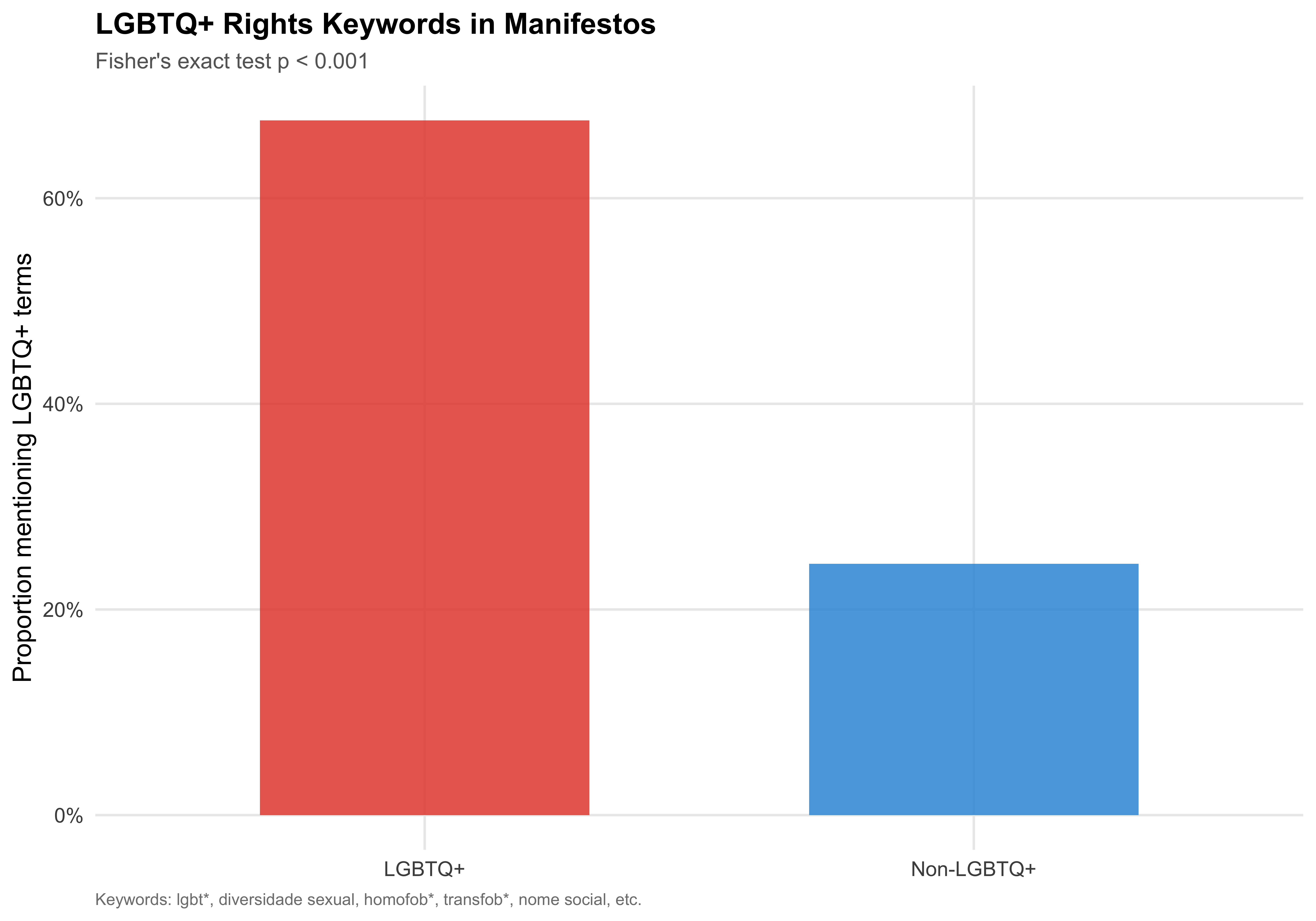
# LGBTQ+ Rights Keywords
Do LGBTQ+ candidates explicitly mention LGBTQ+ rights issues in their manifestos? We search for a targeted set of keywords.
```{r manifesto-lgbtq-keywords}
# Define LGBTQ+ keywords for targeted search
lgbtq_terms <- c(
  "lgbt*", "lgbtq*", "diversidade sexual", "orientação sexual",
  "orientacao sexual", "identidade de gênero", "identidade de genero",
  "homofob*", "transfob*", "travesti*", "transgêner*", "transgenero*",
  "lésbica*", "lesbica*", "bisexual*", "queer", "nome social",
  "orgulho", "arco-íris", "arco-iris"
)

# Search in unstemmed tokens
lgbtq_kwic <- tokens_select(toks, pattern = lgbtq_terms, valuetype = "glob",
                             selection = "keep")

# Count per document
lgbtq_counts <- ntoken(lgbtq_kwic) %>%
  tibble(candidate_id = as.numeric(names(.)), lgbtq_mentions = .) %>%
  mutate(has_lgbtq_mention = lgbtq_mentions > 0)

# Join to mayors
mayors <- mayors %>%
  left_join(lgbtq_counts, by = "candidate_id") %>%
  mutate(
    lgbtq_mentions = replace_na(lgbtq_mentions, 0L),
    has_lgbtq_mention = replace_na(has_lgbtq_mention, FALSE)
  )
```
```{r tbl-lgbtq-keyword-prevalence}
#| label: tbl-lgbtq-keyword-prevalence
#| tbl-cap: "LGBTQ+ Keyword Mentions in Manifestos"
keyword_summary <- mayors %>%
  group_by(lgbtq_label) %>%
  summarise(
    N                  = n(),
    `N with mentions`  = sum(has_lgbtq_mention),
    `% with mentions`  = format_pct(mean(has_lgbtq_mention)),
    `Mean mentions`    = round(mean(lgbtq_mentions), 2),
    `Median mentions`  = median(lgbtq_mentions),
    .groups = "drop"
  ) %>%
  rename(Group = lgbtq_label)

keyword_summary %>% kable(align = c("l", "r", "r", "r", "r", "r"))
save_table(keyword_summary, "07_lgbtq_keywords.csv")
```
```{r fig-lgbtq-keywords}
#| label: fig-lgbtq-keywords
#| fig-cap: "Proportion of Manifestos Mentioning LGBTQ+ Keywords"
# Fisher's exact test
fisher_tbl <- table(mayors$lgbtq_label, mayors$has_lgbtq_mention)
fisher_result <- fisher.test(fisher_tbl)
fisher_p <- format_p(fisher_result$p.value)

keyword_plot <- mayors %>%
  group_by(lgbtq_label) %>%
  summarise(pct = mean(has_lgbtq_mention), .groups = "drop")

ggplot(keyword_plot, aes(x = lgbtq_label, y = pct, fill = lgbtq_label)) +
  geom_col(alpha = 0.85, width = 0.6) +
  scale_y_continuous(labels = label_percent()) +
  scale_fill_manual(values = pal_lgbtq) +
  labs(
    x        = NULL,
    y        = "Proportion mentioning LGBTQ+ terms",
    fill     = NULL,
    title    = "LGBTQ+ Rights Keywords in Manifestos",
    subtitle = paste0("Fisher's exact test p ", fisher_p),
    caption  = "Keywords: lgbt*, diversidade sexual, homofob*, transfob*, nome social, etc."
  ) +
  guides(fill = "none")

save_figure(last_plot(), "07_lgbtq_keyword_prevalence")
```
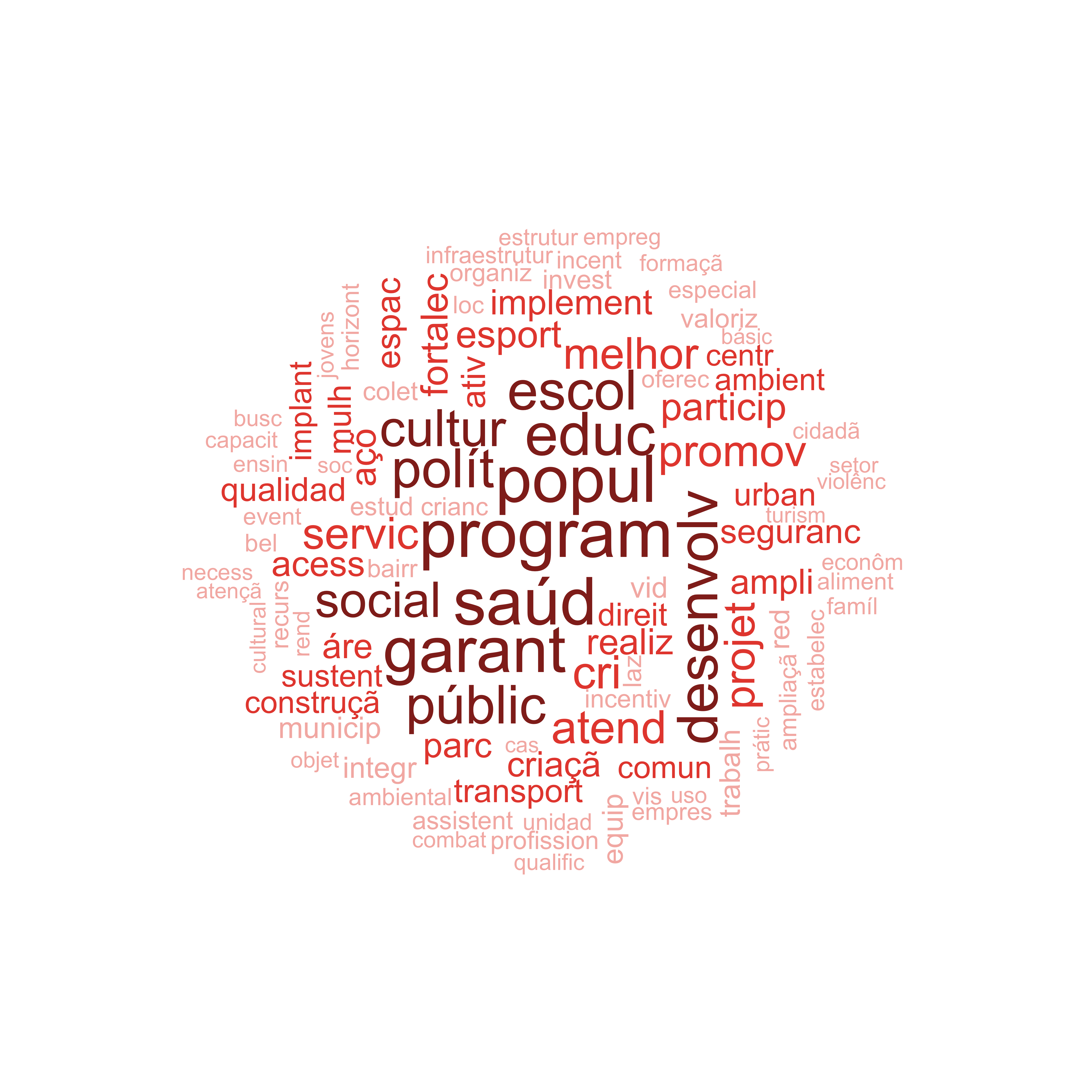
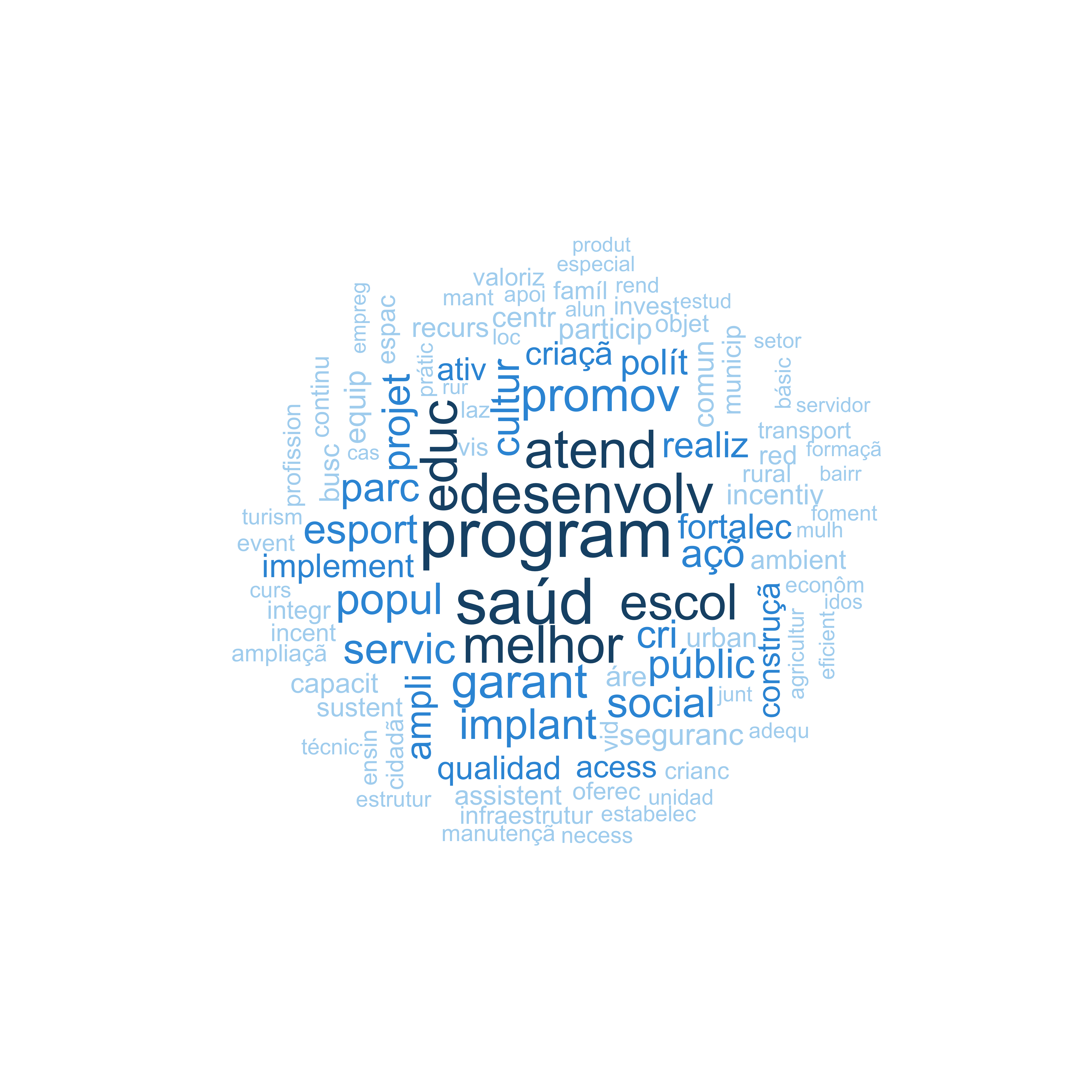
# Comparative Word Clouds
```{r fig-wordcloud-lgbtq}
#| label: fig-wordcloud-lgbtq
#| fig-cap: "Word Cloud: LGBTQ+ Candidate Manifestos"
#| fig-width: 8
#| fig-height: 8
library(wordcloud)

dfm_lgbtq <- dfm_subset(dfm_stem, lgbtq_label == "LGBTQ+")
freq_lgbtq <- textstat_frequency(dfm_lgbtq, n = 100)

set.seed(2024)
wordcloud(
  words     = freq_lgbtq$feature,
  freq      = freq_lgbtq$frequency,
  max.words = 100,
  random.order = FALSE,
  rot.per   = 0.15,
  colors    = c("#F5B7B1", "#E74C3C", "#922B21"),
  scale     = c(3, 0.5)
)

save_figure(last_plot(), "07_wordcloud_lgbtq", width = 8, height = 8)
```
```{r fig-wordcloud-nonlgbtq}
#| label: fig-wordcloud-nonlgbtq
#| fig-cap: "Word Cloud: Non-LGBTQ+ Candidate Manifestos"
#| fig-width: 8
#| fig-height: 8
dfm_nonlgbtq <- dfm_subset(dfm_stem, lgbtq_label == "Non-LGBTQ+")
freq_nonlgbtq <- textstat_frequency(dfm_nonlgbtq, n = 100)

set.seed(2024)
wordcloud(
  words     = freq_nonlgbtq$feature,
  freq      = freq_nonlgbtq$frequency,
  max.words = 100,
  random.order = FALSE,
  rot.per   = 0.15,
  colors    = c("#AED6F1", "#3498DB", "#1A5276"),
  scale     = c(3, 0.5)
)

save_figure(last_plot(), "07_wordcloud_nonlgbtq", width = 8, height = 8)
```
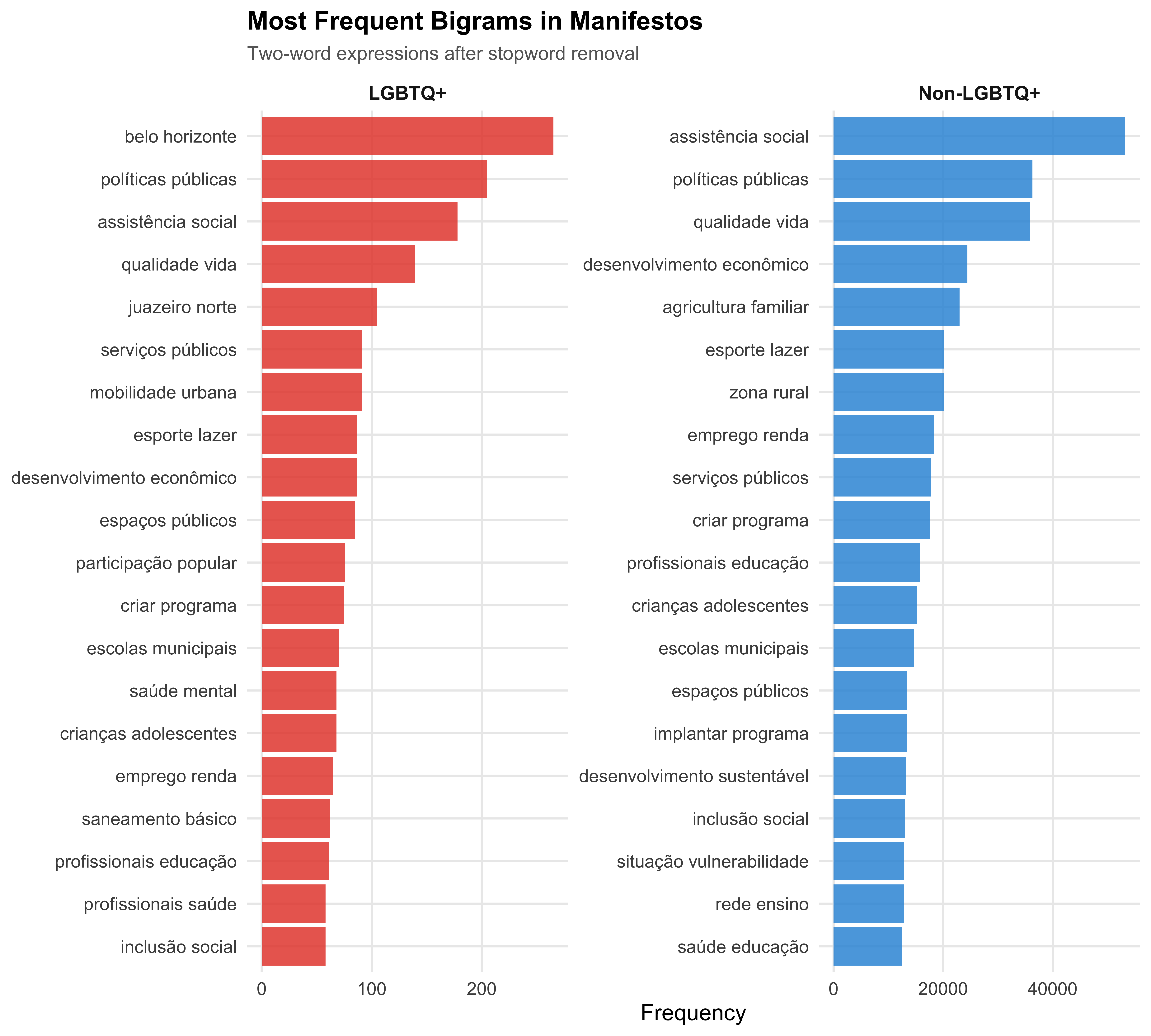
# Bigram Analysis
Single words lose multi-word expressions that carry important meaning in Portuguese political discourse. We examine the most frequent bigrams (two-word sequences) and compare distinctive bigrams across groups.
```{r manifesto-bigrams}
# Create bigrams from the unstemmed, stopword-removed tokens
toks_bigram <- tokens_ngrams(toks, n = 2, concatenator = " ")
dfm_bigram  <- dfm(toks_bigram)
```
```{r fig-bigrams-group}
#| label: fig-bigrams-group
#| fig-cap: "Top 20 Bigrams by LGBTQ+ Status"
#| fig-height: 9
top_bigrams <- textstat_frequency(dfm_bigram, n = 20, groups = lgbtq_label) %>%
  mutate(group = factor(group, levels = c("LGBTQ+", "Non-LGBTQ+")))

ggplot(top_bigrams, aes(x = reorder_within(feature, frequency, group),
                         y = frequency, fill = group)) +
  geom_col(alpha = 0.85, show.legend = FALSE) +
  scale_x_reordered() +
  scale_fill_manual(values = pal_lgbtq) +
  coord_flip() +
  facet_wrap(~ group, scales = "free") +
  labs(
    x     = NULL,
    y     = "Frequency",
    title = "Most Frequent Bigrams in Manifestos",
    subtitle = "Two-word expressions after stopword removal"
  )

save_figure(last_plot(), "07_bigrams_group", height = 9)
```
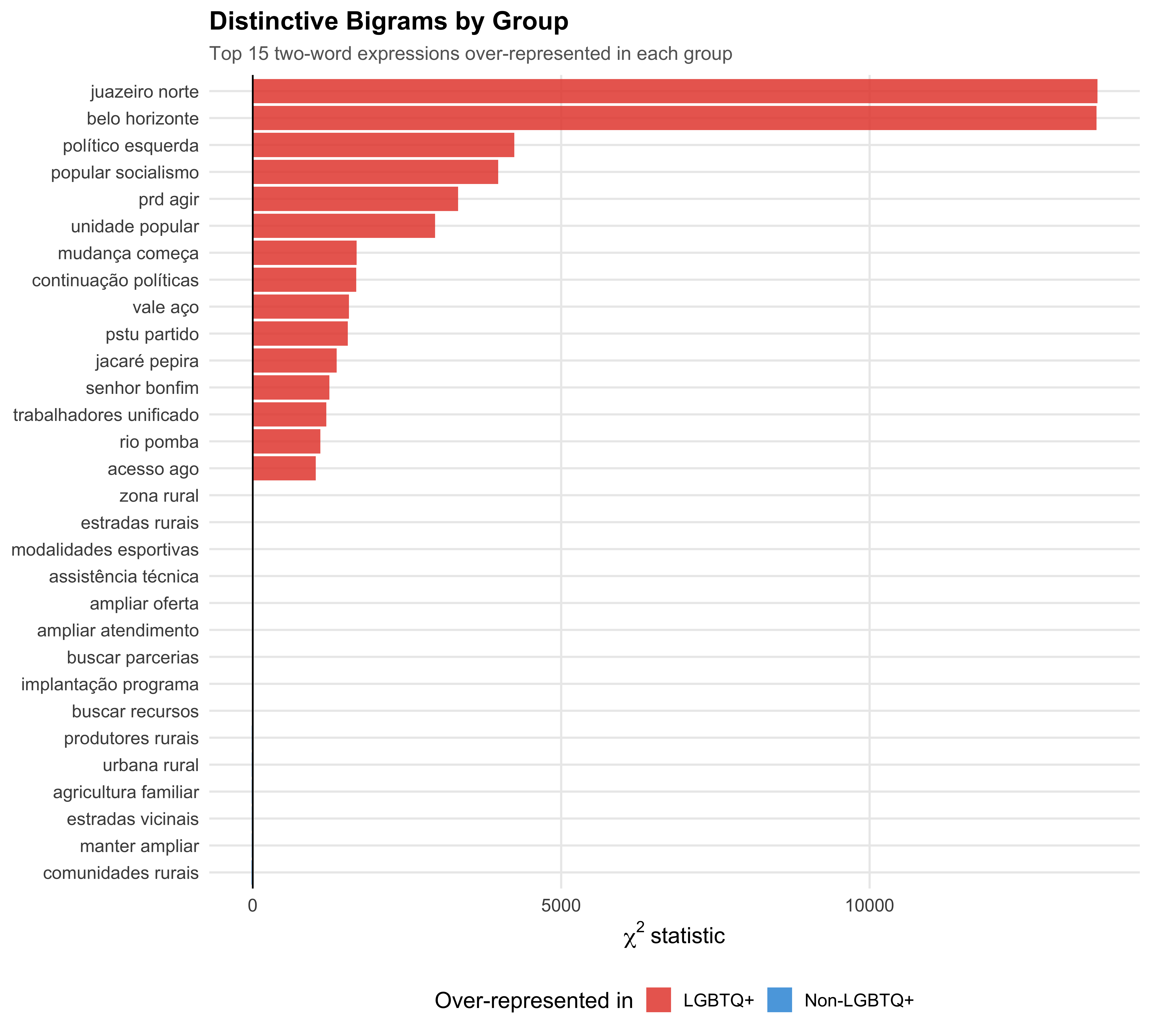
```{r fig-bigram-keyness}
#| label: fig-bigram-keyness
#| fig-cap: "Bigram Keyness: Distinctive Two-Word Expressions"
#| fig-height: 9
# Trim rare bigrams and compute keyness
dfm_bigram_trimmed <- dfm_bigram %>%
  dfm_trim(min_docfreq = 5, docfreq_type = "count")

dfm_bigram_grouped <- dfm_group(dfm_bigram_trimmed, groups = lgbtq_label)
bigram_keyness <- textstat_keyness(dfm_bigram_grouped, target = "LGBTQ+",
                                    measure = "chi2")

top_bi_pos <- bigram_keyness %>% slice_max(chi2, n = 15)
top_bi_neg <- bigram_keyness %>% slice_min(chi2, n = 15)
bi_key_data <- bind_rows(top_bi_pos, top_bi_neg) %>%
  mutate(
    direction = if_else(chi2 > 0, "LGBTQ+", "Non-LGBTQ+"),
    feature   = reorder(feature, chi2)
  )

ggplot(bi_key_data, aes(x = chi2, y = feature, fill = direction)) +
  geom_col(alpha = 0.85) +
  geom_vline(xintercept = 0, linewidth = 0.5) +
  scale_fill_manual(values = pal_lgbtq) +
  labs(
    x        = expression(chi^2 ~ "statistic"),
    y        = NULL,
    fill     = "Over-represented in",
    title    = "Distinctive Bigrams by Group",
    subtitle = "Top 15 two-word expressions over-represented in each group"
  )

save_figure(last_plot(), "07_bigram_keyness", height = 9)
```
<!-- HIDDEN: Sections 10-13 temporarily removed from website output
# Identity-Specific Language
Do Gay, Lesbian, and Trans candidates write different manifestos? We compare keyness *within* the LGBTQ+ subgroup, using each identity category as the target against all other LGBTQ+ candidates.
```{r identity-keyness}
# Subset to LGBTQ+ candidates only
dfm_lgbtq_only <- dfm_subset(dfm_trimmed, lgbtq_label == "LGBTQ+")
# Get identity category for each document
identity_var <- mayors$lgbt_category[match(docnames(dfm_lgbtq_only),
as.character(mayors$candidate_id))]
# Only categories with enough documents (>= 5)
cat_counts <- table(identity_var)
valid_cats <- names(cat_counts[cat_counts >= 5])
```
```{r fig-identity-keyness}
#| label: fig-identity-keyness
#| fig-cap: "Distinctive Words by LGBTQ+ Identity Category (vs. All Other LGBTQ+)"
#| fig-height: 10
# Compute keyness for each identity category vs. all others
identity_key_list <- map_dfr(valid_cats, function(cat) {
dfm_grouped_id <- dfm_group(dfm_lgbtq_only,
groups = if_else(identity_var == cat, cat, "Other"))
tryCatch({
key <- textstat_keyness(dfm_grouped_id, target = cat, measure = "chi2")
key %>%
slice_max(chi2, n = 10) %>%
mutate(category = cat)
}, error = function(e) tibble())
})
if (nrow(identity_key_list) > 0) {
identity_key_list <- identity_key_list %>%
mutate(category = factor(category, levels = names(pal_identity)))
ggplot(identity_key_list, aes(x = chi2,
y = reorder_within(feature, chi2, category),
fill = category)) +
geom_col(alpha = 0.85, show.legend = FALSE) +
scale_y_reordered() +
scale_fill_manual(values = pal_identity) +
facet_wrap(~ category, scales = "free", ncol = 2) +
labs(
x = expression(chi^2),
y = NULL,
title = "Distinctive Vocabulary by Identity Category",
subtitle = "Top 10 words over-represented vs. all other LGBTQ+ candidates"
)
save_figure(last_plot(), "07_identity_keyness", height = 10)
}
```
# Electoral Outcomes and Manifestos
Do manifesto characteristics differ between winners and losers? We compare elected and non-elected candidates on manifesto length, complexity, and policy emphasis.
```{r manifesto-electoral-setup}
# Add elected status
mayors_elected <- mayors %>%
filter(!is.na(elected)) %>%
mutate(outcome = if_else(elected, "Elected", "Not Elected"))
```
```{r tbl-manifesto-outcome}
#| label: tbl-manifesto-outcome
#| tbl-cap: "Manifesto Characteristics by Electoral Outcome"
outcome_stats <- mayors_elected %>%
group_by(outcome) %>%
summarise(
N = n(),
`Median Words` = format_n(median(manifesto_n_words, na.rm = TRUE)),
`Mean Words` = format_n(round(mean(manifesto_n_words, na.rm = TRUE))),
`Median Flesch` = round(median(flesch, na.rm = TRUE), 1),
`Median CTTR` = round(median(cttr, na.rm = TRUE), 3),
.groups = "drop"
)
outcome_stats %>% kable(align = c("l", "r", "r", "r", "r", "r"))
save_table(outcome_stats, "07_manifesto_outcome.csv")
```
```{r fig-words-outcome}
#| label: fig-words-outcome
#| fig-cap: "Manifesto Length by Electoral Outcome and LGBTQ+ Status"
ggplot(mayors_elected, aes(x = outcome, y = manifesto_n_words,
fill = lgbtq_label)) +
geom_boxplot(alpha = 0.7, outlier.alpha = 0.2) +
scale_y_log10(labels = label_comma()) +
scale_fill_manual(values = pal_lgbtq) +
labs(
x = NULL,
y = "Word Count (log scale)",
fill = NULL,
title = "Manifesto Length and Electoral Success",
subtitle = "Do winners write longer manifestos?"
)
save_figure(last_plot(), "07_words_outcome")
```
```{r fig-salience-outcome}
#| label: fig-salience-outcome
#| fig-cap: "Policy Salience: Elected vs Non-Elected Candidates"
#| fig-height: 8
# Compute salience by outcome
dict_with_outcome <- dict_results %>%
left_join(
mayors_elected %>% select(candidate_id, outcome),
by = c("doc_id" = "candidate_id")
) %>%
filter(!is.na(outcome))
salience_outcome <- dict_with_outcome %>%
group_by(outcome, domain_label) %>%
summarise(mean_sal = mean(salience, na.rm = TRUE), .groups = "drop")
ggplot(salience_outcome, aes(x = mean_sal, y = domain_label,
color = outcome)) +
geom_line(aes(group = domain_label), color = "grey70", linewidth = 0.8) +
geom_point(size = 3.5) +
scale_x_continuous(labels = label_percent()) +
scale_color_manual(values = c("Elected" = "#2ECC71", "Not Elected" = "#E74C3C")) +
labs(
x = "Mean Salience",
y = NULL,
color = NULL,
title = "Policy Emphasis and Electoral Outcomes",
subtitle = "Do winning candidates emphasize different policy domains?"
)
save_figure(last_plot(), "07_salience_outcome", height = 8)
```
```{r fig-lgbtq-mention-outcome}
#| label: fig-lgbtq-mention-outcome
#| fig-cap: "LGBTQ+ Keyword Mentions and Electoral Outcome (LGBTQ+ Candidates Only)"
lgbtq_outcome <- mayors_elected %>%
filter(lgbtq_candidate)
if (nrow(lgbtq_outcome) >= 5) {
outcome_mention <- lgbtq_outcome %>%
group_by(outcome) %>%
summarise(
n = n(),
pct_mention = mean(has_lgbtq_mention),
mean_mentions = mean(lgbtq_mentions),
.groups = "drop"
)
ggplot(outcome_mention, aes(x = outcome, y = pct_mention, fill = outcome)) +
geom_col(alpha = 0.85, width = 0.6) +
geom_text(aes(label = paste0("n=", n)), vjust = -0.5, size = 4) +
scale_y_continuous(labels = label_percent(), limits = c(0, NA)) +
scale_fill_manual(values = c("Elected" = "#2ECC71", "Not Elected" = "#E74C3C")) +
labs(
x = NULL,
y = "% mentioning LGBTQ+ terms",
fill = NULL,
title = "Do LGBTQ+ Winners Mention LGBTQ+ Rights?",
subtitle = "Among LGBTQ+ mayoral candidates only"
) +
guides(fill = "none")
save_figure(last_plot(), "07_lgbtq_mention_outcome")
}
```
::: {.callout-note}
## Electoral Outcome Caveats
Electoral success depends on many factors beyond manifesto content (incumbency, party strength, campaign resources, name recognition). These comparisons do not imply that manifesto characteristics *cause* electoral outcomes. They simply describe whether winners and losers tend to produce different types of documents.
:::
# Regional Variation
Brazilian regions vary enormously in political culture, economic development, and LGBTQ+ acceptance. We examine how manifesto content varies across regions, particularly for LGBTQ+ candidates.
```{r fig-salience-region}
#| label: fig-salience-region
#| fig-cap: "Policy Salience by Region (All Candidates)"
#| fig-height: 9
salience_region <- dict_results %>%
filter(!is.na(region)) %>%
group_by(region, domain_label) %>%
summarise(mean_sal = mean(salience, na.rm = TRUE), .groups = "drop")
ggplot(salience_region, aes(x = mean_sal, y = domain_label, color = region)) +
geom_point(size = 3, alpha = 0.8) +
scale_x_continuous(labels = label_percent()) +
scale_color_manual(values = pal_region) +
labs(
x = "Mean Salience",
y = NULL,
color = "Region",
title = "Policy Emphasis by Region",
subtitle = "Do regions prioritize different policy domains?"
)
save_figure(last_plot(), "07_salience_region", height = 9)
```
```{r fig-words-region}
#| label: fig-words-region
#| fig-cap: "Manifesto Length by Region and LGBTQ+ Status"
ggplot(mayors %>% filter(!is.na(region)),
aes(x = region, y = manifesto_n_words, fill = lgbtq_label)) +
geom_boxplot(alpha = 0.7, outlier.alpha = 0.2) +
scale_y_log10(labels = label_comma()) +
scale_fill_manual(values = pal_lgbtq) +
labs(
x = NULL,
y = "Word Count (log scale)",
fill = NULL,
title = "Manifesto Length by Region",
subtitle = "LGBTQ+ vs Non-LGBTQ+ candidates across regions"
) +
theme(axis.text.x = element_text(angle = 30, hjust = 1))
save_figure(last_plot(), "07_words_region")
```
```{r tbl-lgbtq-keywords-region}
#| label: tbl-lgbtq-keywords-region
#| tbl-cap: "LGBTQ+ Keyword Mentions by Region (All Candidates)"
region_keywords <- mayors %>%
filter(!is.na(region)) %>%
group_by(region) %>%
summarise(
N = n(),
`% mentioning` = format_pct(mean(has_lgbtq_mention)),
`Mean mentions` = round(mean(lgbtq_mentions), 2),
.groups = "drop"
)
region_keywords %>% kable(align = c("l", "r", "r", "r"))
save_table(region_keywords, "07_lgbtq_keywords_region.csv")
```
# Summary
This chapter examined `r format_n(n_mayors)` mayoral candidate manifestos through the lens of quantitative text analysis, comparing the `r format_n(n_lgbtq)` LGBTQ+ candidates against the broader population of `r format_n(n_nonlgbtq)` non-LGBTQ+ candidates.
**Corpus characteristics**: LGBTQ+ candidate manifestos are `r word_direction` than their non-LGBTQ+ counterparts (median `r format_n(median_words_lgbtq)` vs `r format_n(median_words_nonlgbtq)` words).
**Text complexity**: Readability and lexical diversity comparisons provide insight into whether LGBTQ+ candidates write differently at the stylistic level, though interpretation requires caution given the small sample.
**Policy emphasis**: The custom Portuguese-language dictionary reveals whether LGBTQ+ candidates place differential emphasis on specific policy domains --- education, health, security, economy, social policy, environment, infrastructure, LGBTQ+ rights, culture, and transparency.
**Structural topics**: The STM identifies latent themes and estimates the marginal effect of LGBTQ+ status on topic prevalence, controlling for ideology and region. With only `r format_n(n_lgbtq)` LGBTQ+ documents, these coefficients carry substantial uncertainty and should be treated as suggestive rather than definitive.
**LGBTQ+ rights keywords**: The targeted keyword search reveals whether LGBTQ+ candidates are more likely to explicitly reference LGBTQ+ rights issues in their official platform documents.
**Bigrams and identity-specific language**: Multi-word expression analysis uncovers distinctive two-word phrases, while within-group keyness reveals how Gay, Lesbian, and Trans candidates differ in their policy vocabulary.
**Electoral outcomes**: Comparisons between elected and non-elected candidates on manifesto length, complexity, and policy emphasis explore whether manifesto characteristics correlate with electoral success.
**Regional variation**: Geographic breakdowns reveal how manifesto content and LGBTQ+ keyword prevalence vary across Brazil's five macro-regions.
All findings in this chapter are descriptive. The small LGBTQ+ sample precludes strong inferential claims but reveals patterns that merit investigation as LGBTQ+ political representation grows in future elections.
END HIDDEN: Sections 10-13 -->