---
title: "3. L-G-B-T Disaggregation"
subtitle: "Within-Group Heterogeneity Among LGBTQ+ Candidates"
---
```{r setup}
source(here::here("code", "00_setup.R"))
library(ggridges)

df <- readRDS(paths$analysis_full_rds)
df <- df %>%
  mutate(ideology_category = factor(ideology_category, levels = ideology_levels))

# Working subsets
lgbtq <- df %>% filter(lgbtq_candidate)
n_lgbtq <- nrow(lgbtq)

# Categories used in comparative analyses (excluding "Other LGBTQ+", N=12, too small for reliable estimates)
analysis_categories <- c("Gay", "Lesbian", "Bisexual+", "Trans", "Asexual")
main_categories <- c("Gay", "Lesbian", "Bisexual+", "Trans")
```
# Overview
The previous chapter treated LGBTQ+ candidates as a single group. That is a useful starting point, but it conceals profound differences. A gay white man running for city council in São Paulo on a center-left ticket inhabits a very different political reality than a trans Black woman running in a small Northeastern municipality for a left-wing party.
This chapter **disaggregates** the LGBTQ+ umbrella into its constituent identity categories and asks: How do Gay, Lesbian, Bisexual+, and Trans candidates differ from one another --- in demographics, political positioning, party affiliation, and electoral success?
The analysis focuses on the `r format_n(n_lgbtq)` LGBTQ+ candidates identified in the dataset.
::: {.callout-note}
## Results by Position Type
As in Chapter 2, disaggregated analyses are presented separately for **city councilors** (proportional representation) and **mayors/vice-mayors** (plurality/majority) using tabbed panels. Because this chapter further splits by identity category, cell sizes become small for executive positions --- the Mayors & Vice-Mayors tab carries a small-N warning, and some visualizations are simplified accordingly.
:::
# Identity Categories {#sec-categories}
## Category Construction
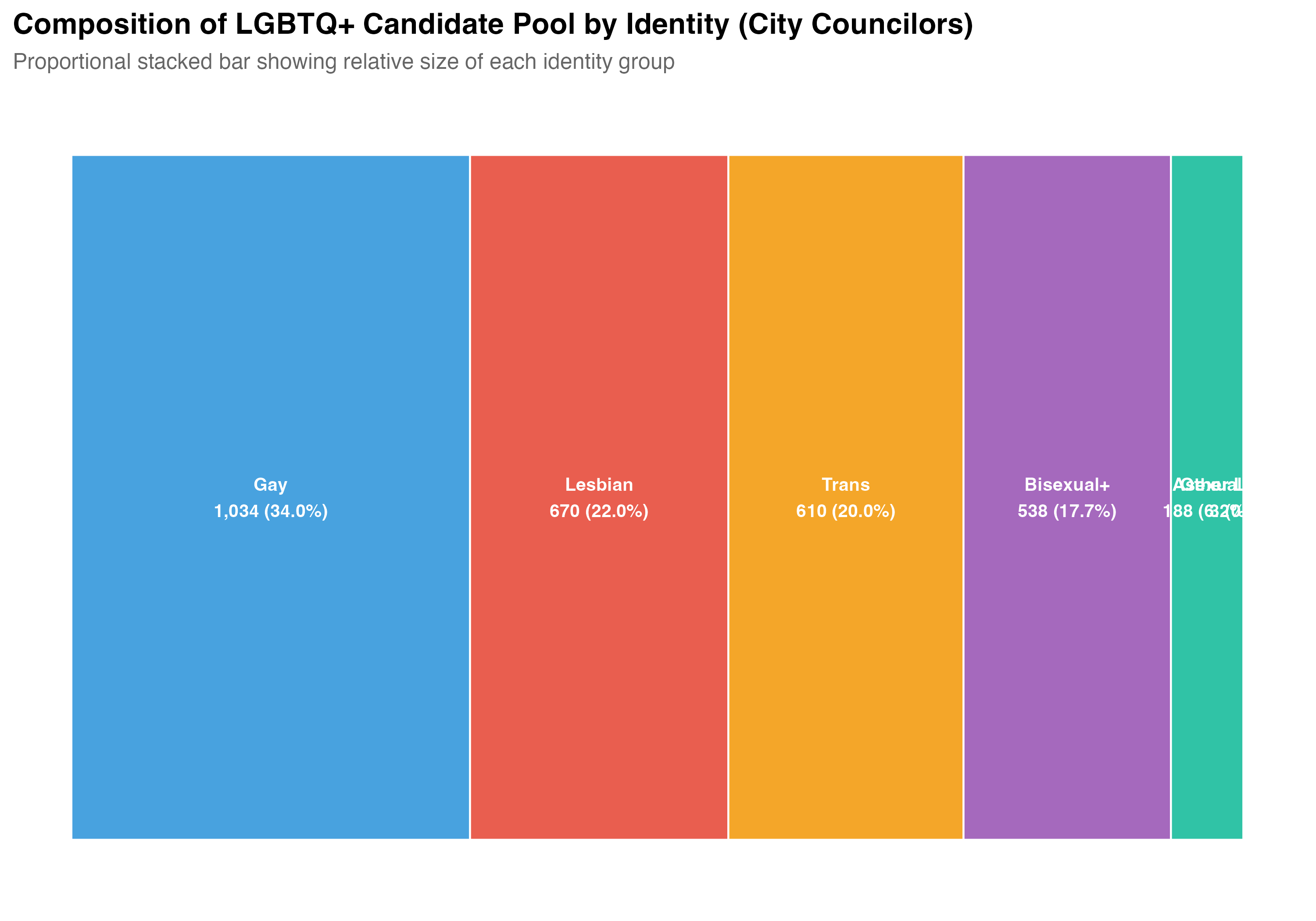
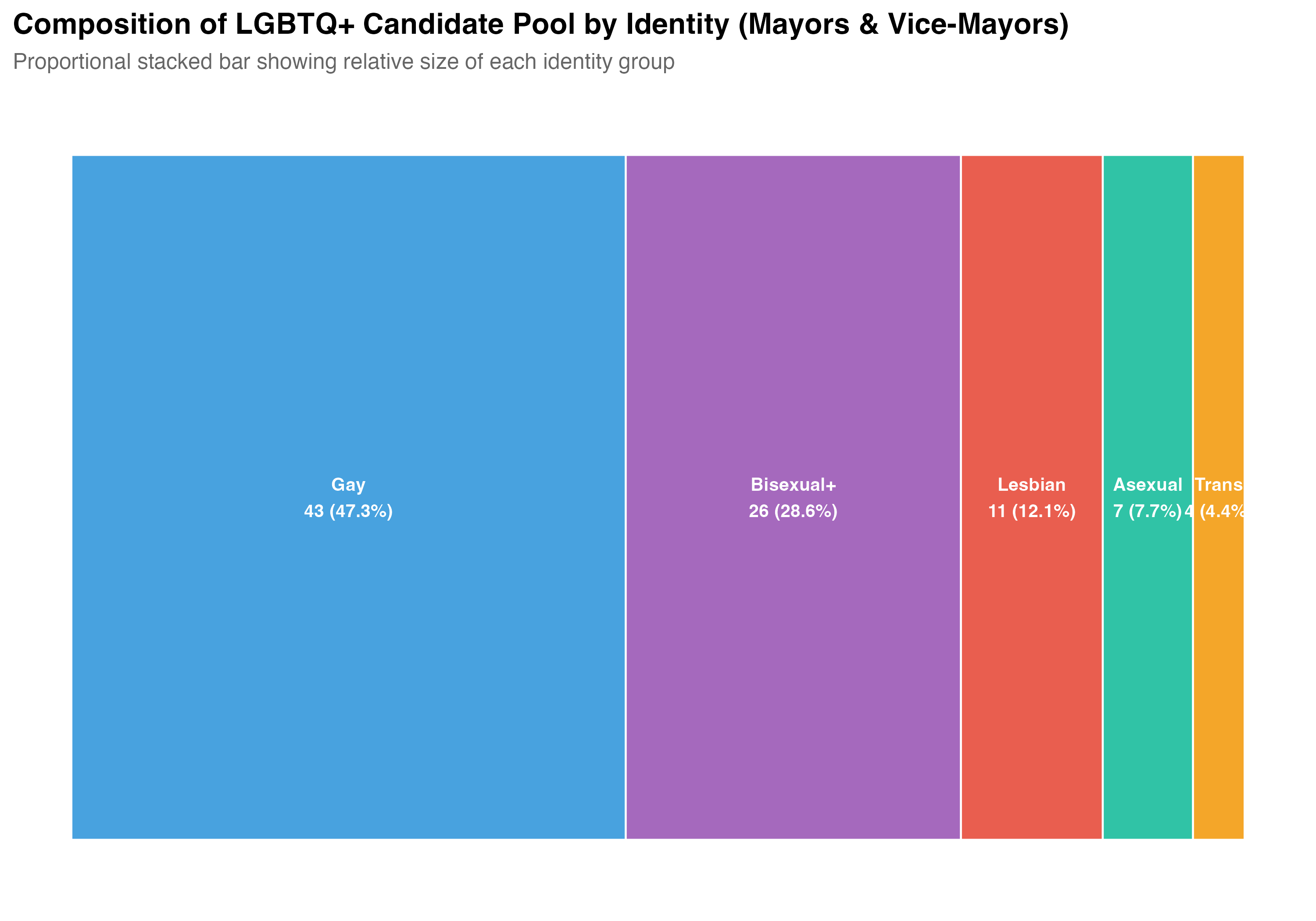
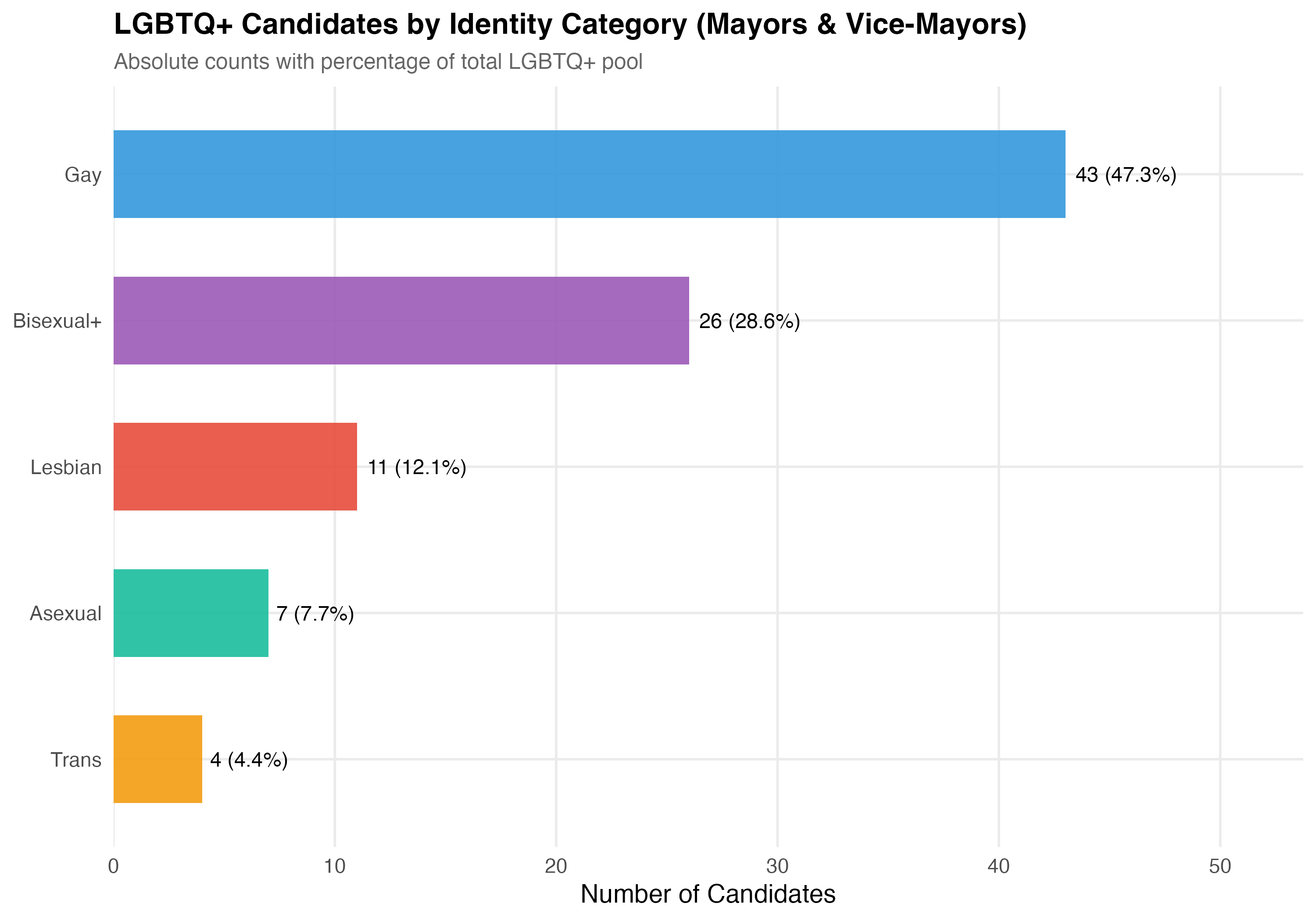
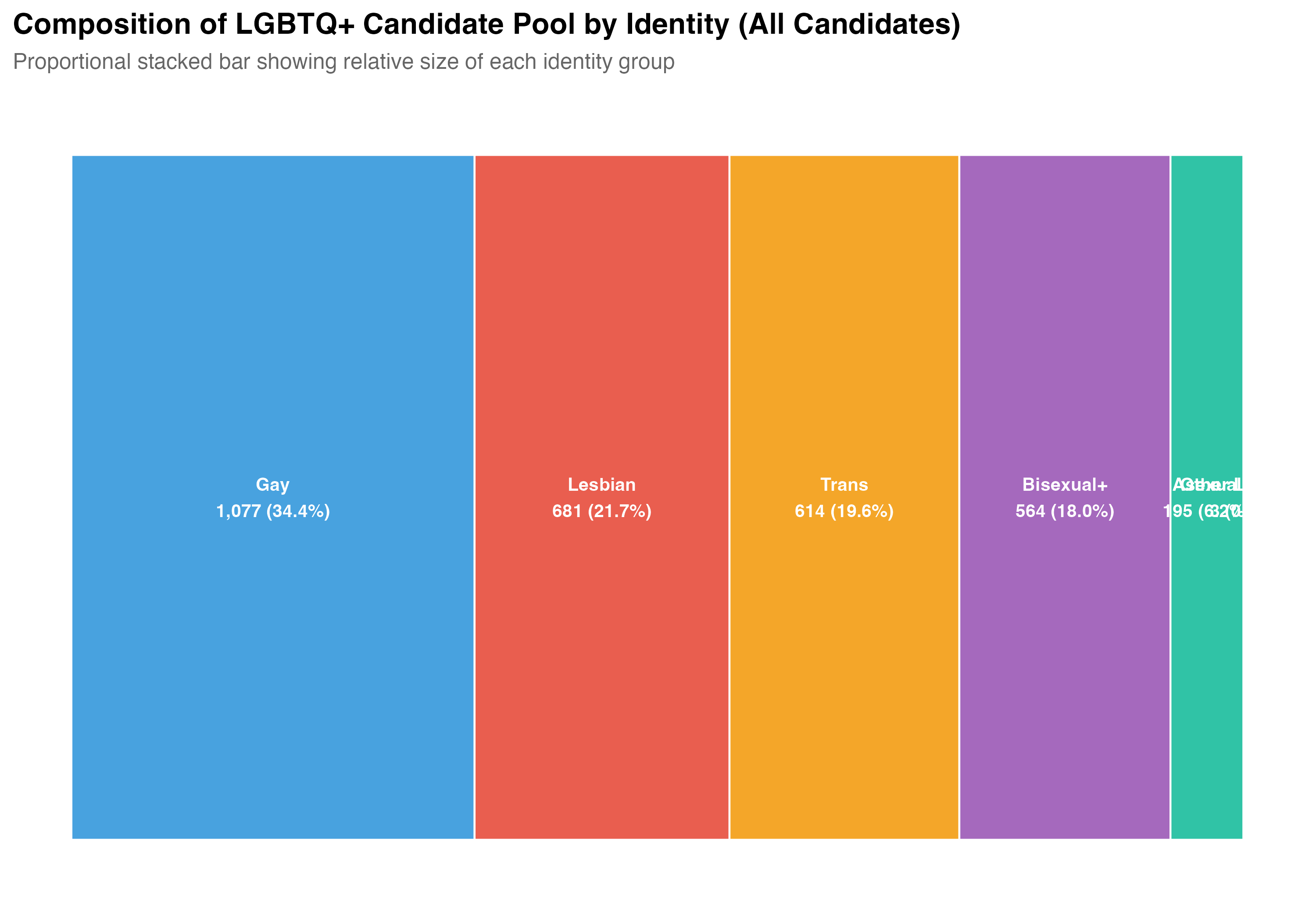
The `lgbt_category` variable classifies each LGBTQ+ candidate into one of six categories: **Gay**, **Lesbian**, **Bisexual+** (including bisexual and pansexual), **Trans** (transgender and travesti), **Asexual**, and **Other LGBTQ+** (candidates identified as LGBTQ+ but without a more specific classification).
::: {.callout-note}
## Classification Rule: Trans Takes Priority
A key coding decision: **trans identity is prioritized over sexual orientation**. A candidate who identifies as both transgender and lesbian is classified as "Trans," not "Lesbian." This reflects the sociological logic that gender identity is typically the more salient axis of political visibility and discrimination. The alternative coding (prioritizing sexual orientation) would obscure the experiences of trans candidates who also hold non-heterosexual orientations --- which is the majority of trans candidates.
:::
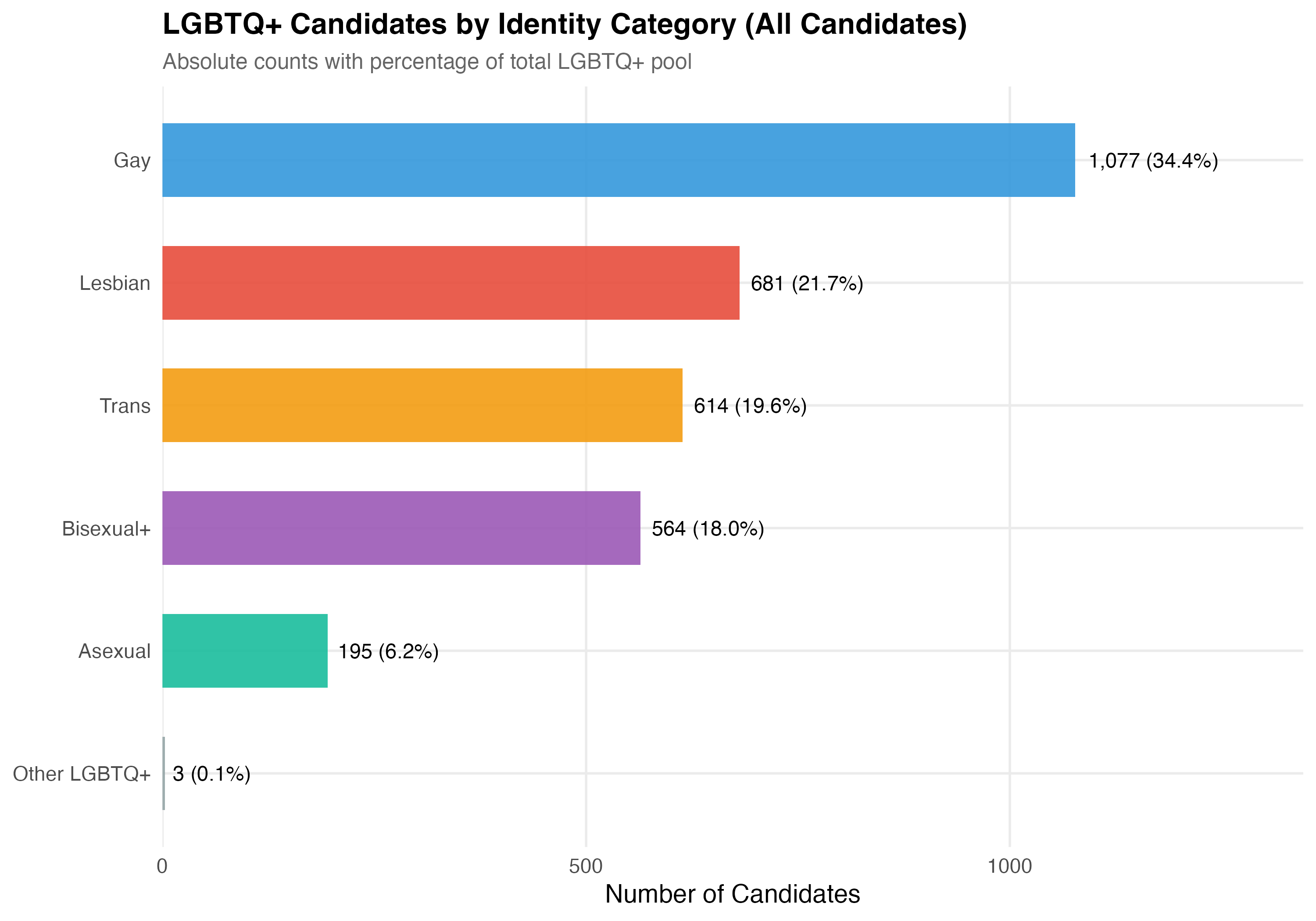
## Distribution of Identity Categories
The `lgbt_category` variable classifies each LGBTQ+ candidate based on a combination of TSE self-reported sexual orientation/gender identity and VOTE LGBT records. Trans identity is prioritized over sexual orientation (see note above). The table below reports the count and cumulative share of each category.
```{r identity-tabset}
#| results: asis
render_identity <- function(data, tab_name) {
  lgbtq_pos <- data %>% filter(lgbtq_candidate)

  # --- Count table ---
  cat("### Count Table\n\n")

  identity_counts <- lgbtq_pos %>%
    count(lgbt_category, sort = TRUE) %>%
    mutate(
      pct = n / sum(n),
      pct_fmt = format_pct(pct),
      cum_pct = format_pct(cumsum(pct))
    )

  identity_counts %>%
    select(Category = lgbt_category, N = n, `%` = pct_fmt, `Cumulative %` = cum_pct) %>%
    cat_kable(align = c("l", "r", "r", "r"))

  # --- Composition chart ---
  cat("### Composition Chart\n\n")

  p_waffle <- lgbtq_pos %>%
    count(lgbt_category) %>%
    mutate(
      pct = n / sum(n),
      label = paste0(lgbt_category, "\n", format_n(n), " (", format_pct(pct), ")")
    ) %>%
    arrange(desc(n)) %>%
    mutate(lgbt_category = fct_reorder(lgbt_category, n)) %>%
    ggplot(aes(x = "", y = pct, fill = lgbt_category)) +
    geom_col(width = 1, alpha = 0.9, color = "white", linewidth = 0.5) +
    geom_text(
      aes(label = label),
      position = position_stack(vjust = 0.5),
      size = 3.5, color = "white", fontface = "bold"
    ) +
    coord_flip() +
    scale_fill_manual(values = pal_identity, guide = "none") +
    labs(
      x = NULL, y = NULL,
      title = paste0("Composition of LGBTQ+ Candidate Pool by Identity (", tab_name, ")"),
      subtitle = "Proportional stacked bar showing relative size of each identity group"
    ) +
    theme(
      axis.text = element_blank(),
      axis.ticks = element_blank(),
      panel.grid = element_blank()
    )
  cat_plot(p_waffle, paste0("03-identity-waffle-", pos_suffix(tab_name)))

  # --- Category counts ---
  cat("### Category Counts\n\n")

  p_bar <- lgbtq_pos %>%
    count(lgbt_category) %>%
    mutate(
      pct = n / sum(n),
      label = paste0(format_n(n), " (", format_pct(pct), ")")
    ) %>%
    ggplot(aes(x = reorder(lgbt_category, n), y = n, fill = lgbt_category)) +
    geom_col(alpha = 0.9, show.legend = FALSE, width = 0.6) +
    geom_text(aes(label = label), hjust = -0.1, size = 4) +
    coord_flip() +
    scale_y_continuous(expand = expansion(mult = c(0, 0.25))) +
    scale_fill_manual(values = pal_identity) +
    labs(
      x = NULL, y = "Number of Candidates",
      title = paste0("LGBTQ+ Candidates by Identity Category (", tab_name, ")"),
      subtitle = "Absolute counts with percentage of total LGBTQ+ pool"
    )
  cat_plot(p_bar, paste0("03-identity-bar-", pos_suffix(tab_name)))
}

render_position_tabset(render_identity, df)
```
::: {.callout-note}
## Analytical Sample
The "Other LGBTQ+" category contains only `r format_n(sum(lgbtq$lgbt_category == "Other LGBTQ+"))` candidates --- too few for reliable statistical comparisons. All subsequent analyses in this chapter exclude this category and focus on the five substantive identity groups: Gay, Lesbian, Bisexual+, Trans, and Asexual. The descriptive count tables above include all candidates for completeness.
:::
# Demographic Profiles {#sec-demographics}
## Multi-Column Comparison Table
The table below compares the identity groups on core demographics: mean age, gender composition (% female), racial breakdown (% Nonwhite, White, Black, Brown), and educational attainment (% College+). All variables are defined as in Chapter 1. Smaller categories (Asexual, Other LGBTQ+) are included for completeness but should be interpreted with caution given their smaller sample sizes.
```{r demographics-tabset}
#| results: asis
render_demographics_03 <- function(data, tab_name) {
lgbtq_pos <- data %>% filter(lgbtq_candidate)
# --- Summary table ---
cat("### Demographic Summary\n\n")
demo_by_id <- lgbtq_pos %>%
filter(lgbt_category %in% analysis_categories) %>%
group_by(lgbt_category) %>%
summarise(
N = n(),
`Mean Age` = round(mean(age, na.rm = TRUE), 1),
`SD Age` = round(sd(age, na.rm = TRUE), 1),
`% Female` = format_pct(mean(female, na.rm = TRUE)),
`% Nonwhite` = format_pct(mean(nonwhite, na.rm = TRUE)),
`% White` = format_pct(mean(race_simple == "White", na.rm = TRUE)),
`% Black` = format_pct(mean(race_simple == "Black", na.rm = TRUE)),
`% Brown` = format_pct(mean(race_simple == "Brown", na.rm = TRUE)),
`% College+` = format_pct(mean(education_simple == "College+", na.rm = TRUE)),
.groups = "drop"
) %>%
rename(Category = lgbt_category)
demo_by_id %>%
mutate(N = format_n(N)) %>%
cat_kable(align = c("l", "r", "r", "r", "r", "r", "r", "r", "r", "r"))
# --- Age boxplot ---
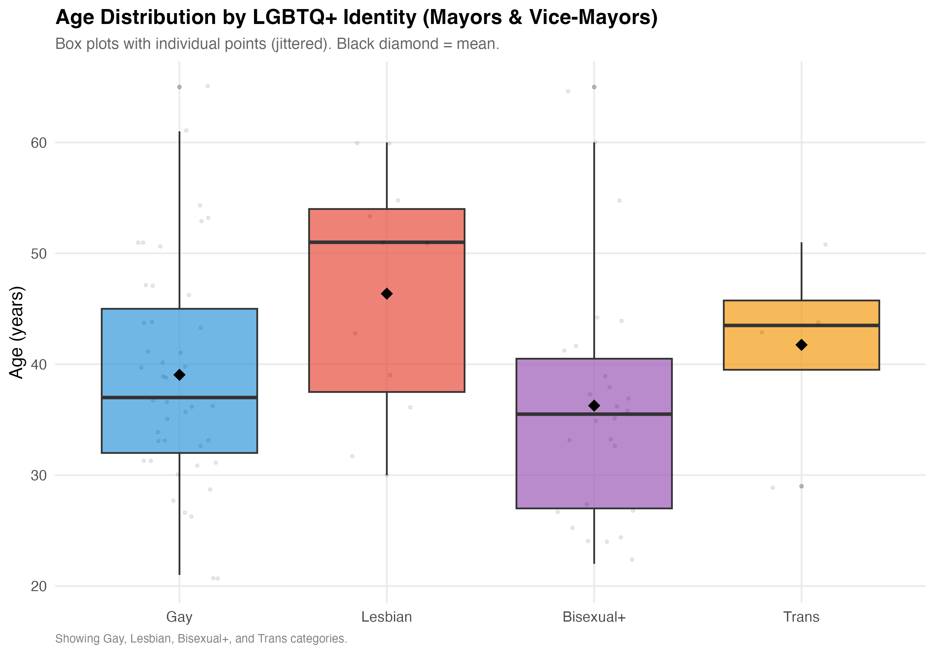
cat("### Age Distribution\n\n")
p_age <- lgbtq_pos %>%
filter(lgbt_category %in% main_categories, !is.na(age)) %>%
mutate(lgbt_category = factor(lgbt_category, levels = main_categories)) %>%
ggplot(aes(x = lgbt_category, y = age, fill = lgbt_category)) +
geom_boxplot(alpha = 0.7, outlier.alpha = 0.3, outlier.size = 1) +
geom_jitter(alpha = 0.08, width = 0.2, size = 0.8) +
stat_summary(fun = mean, geom = "point", shape = 18, size = 4, color = "black") +
scale_fill_manual(values = pal_identity, guide = "none") +
labs(
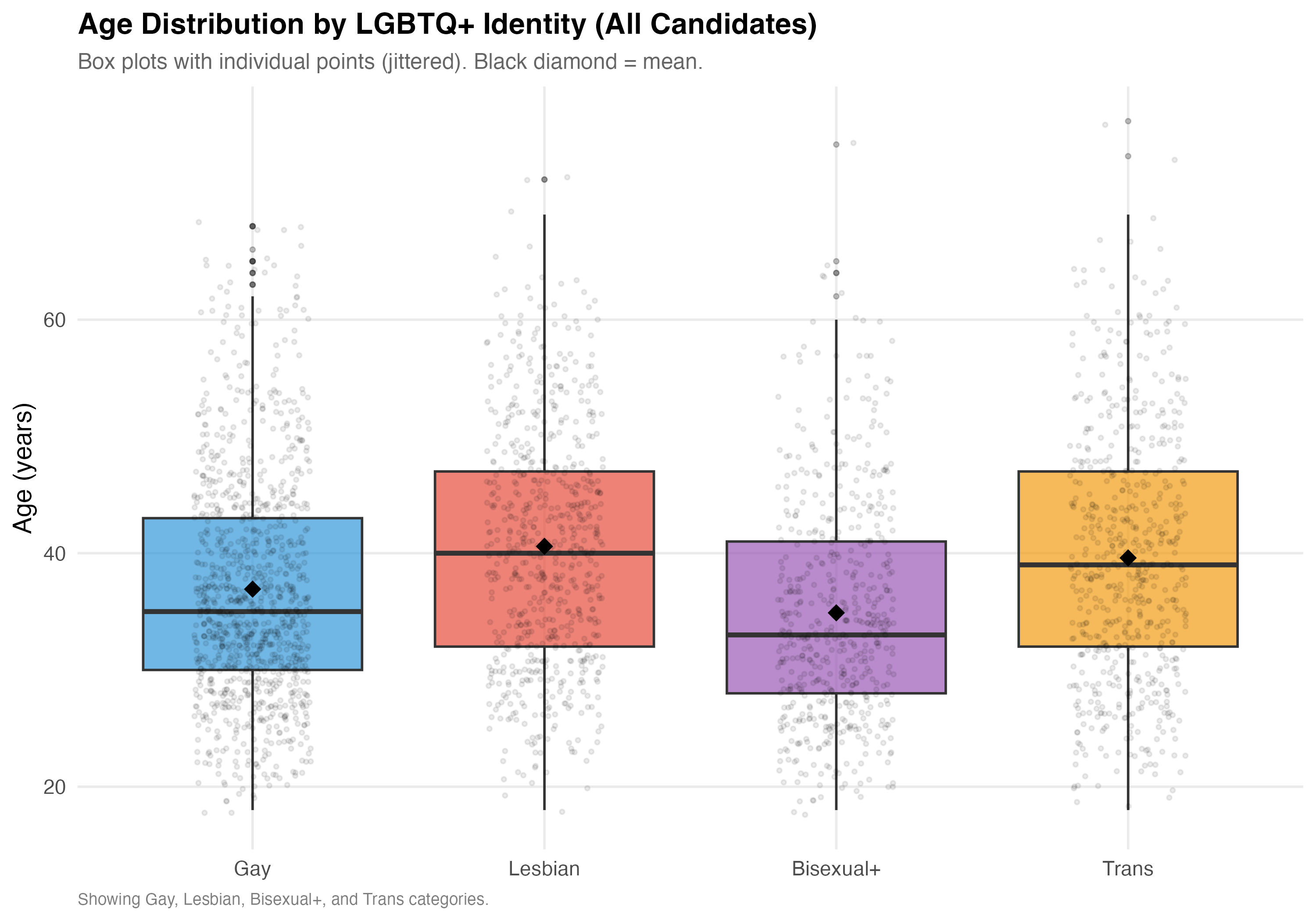
x = NULL, y = "Age (years)",
title = paste0("Age Distribution by LGBTQ+ Identity (", tab_name, ")"),
subtitle = "Box plots with individual points (jittered). Black diamond = mean.",
caption = "Showing Gay, Lesbian, Bisexual+, and Trans categories."
)
cat_plot(p_age, paste0("03-age-boxplot-", pos_suffix(tab_name)))
# --- Race ---
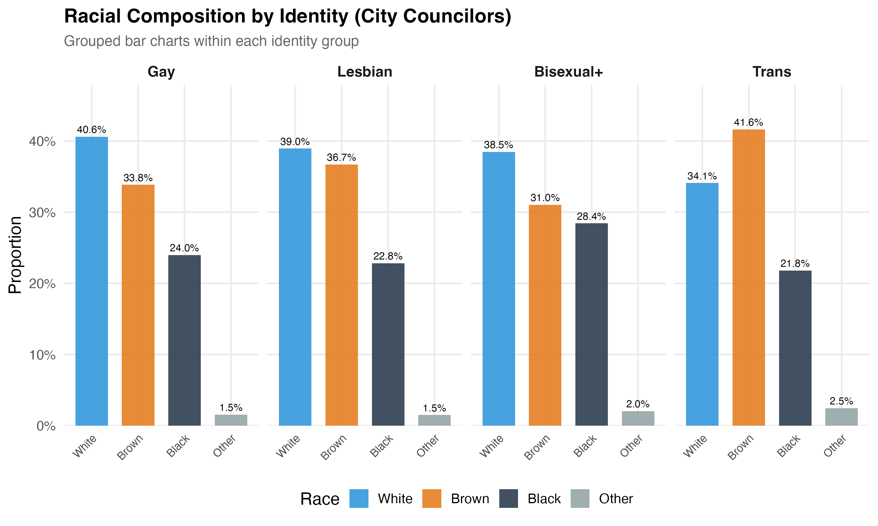
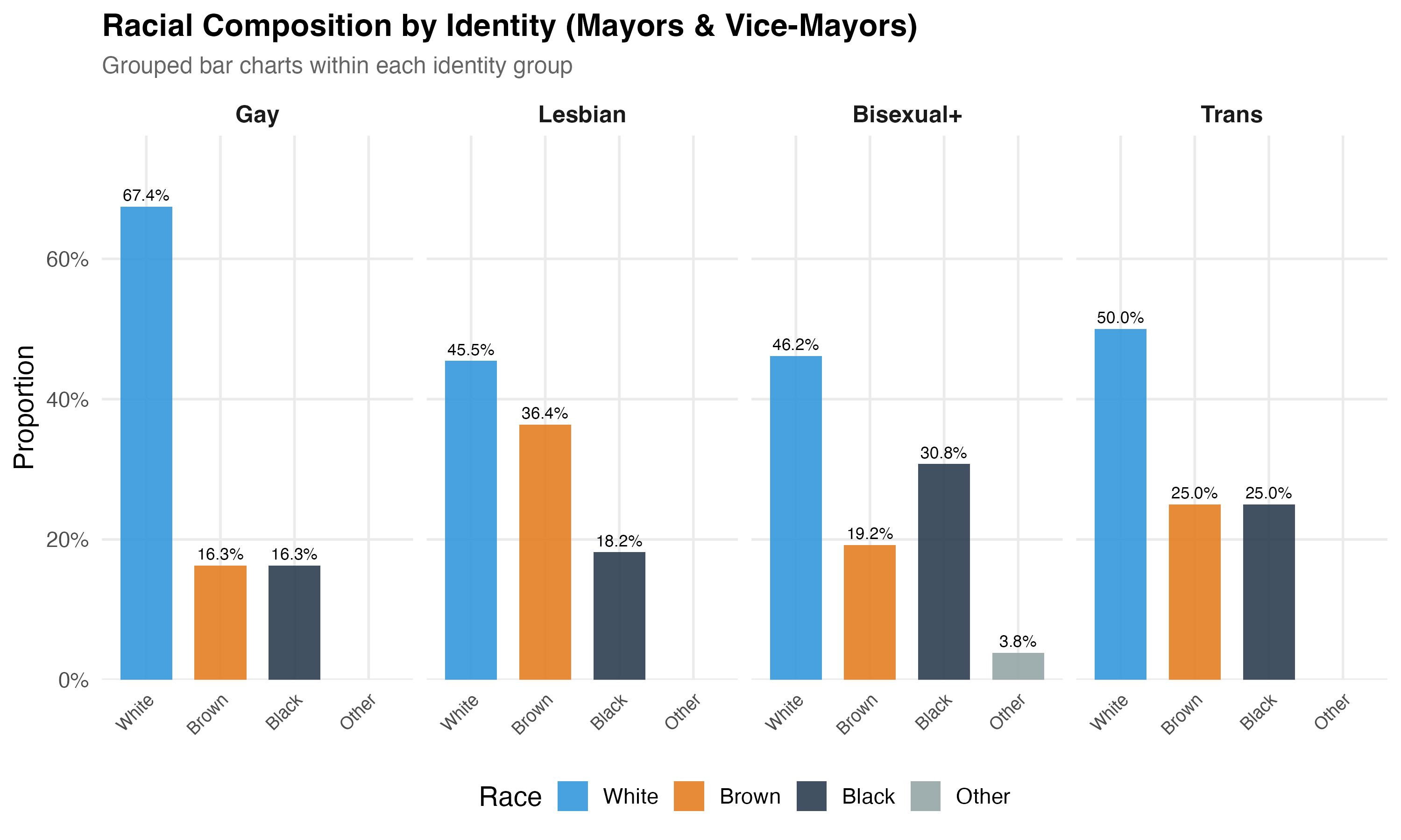
cat("### Race by Identity\n\n")
p_race <- lgbtq_pos %>%
filter(lgbt_category %in% main_categories, !is.na(race_simple)) %>%
mutate(lgbt_category = factor(lgbt_category, levels = main_categories)) %>%
count(lgbt_category, race_simple) %>%
group_by(lgbt_category) %>%
mutate(pct = n / sum(n)) %>%
ungroup() %>%
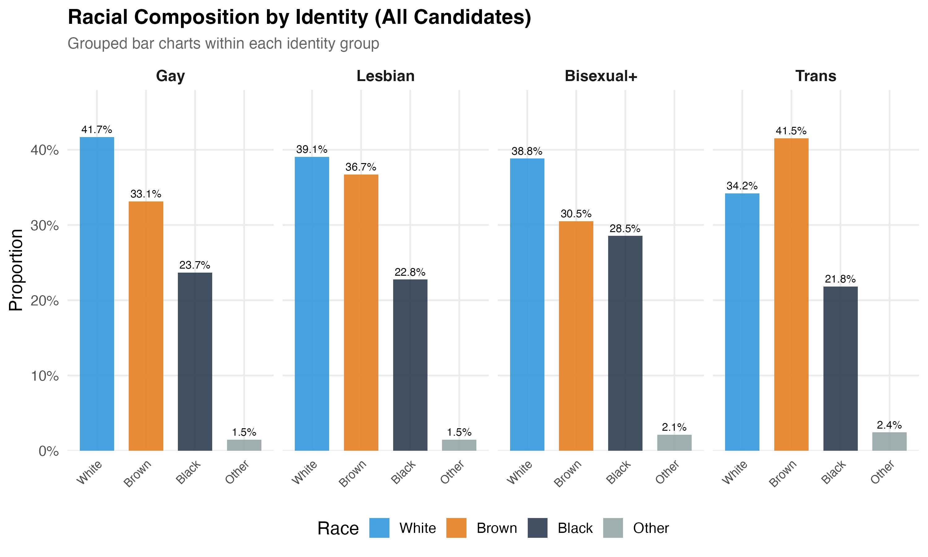
ggplot(aes(x = race_simple, y = pct, fill = race_simple)) +
geom_col(alpha = 0.9, width = 0.7) +
geom_text(aes(label = format_pct(pct)), vjust = -0.5, size = 3) +
facet_wrap(~lgbt_category, nrow = 1) +
scale_y_continuous(labels = percent, expand = expansion(mult = c(0, 0.15))) +
scale_fill_manual(values = pal_race, name = "Race") +
labs(
x = NULL, y = "Proportion",
title = paste0("Racial Composition by Identity (", tab_name, ")"),
subtitle = "Grouped bar charts within each identity group"
) +
theme(axis.text.x = element_text(angle = 45, hjust = 1, size = 9))
cat_plot(p_race, paste0("03-race-by-identity-", pos_suffix(tab_name)), height = 6)
# --- Education ---
cat("### Education by Identity\n\n")
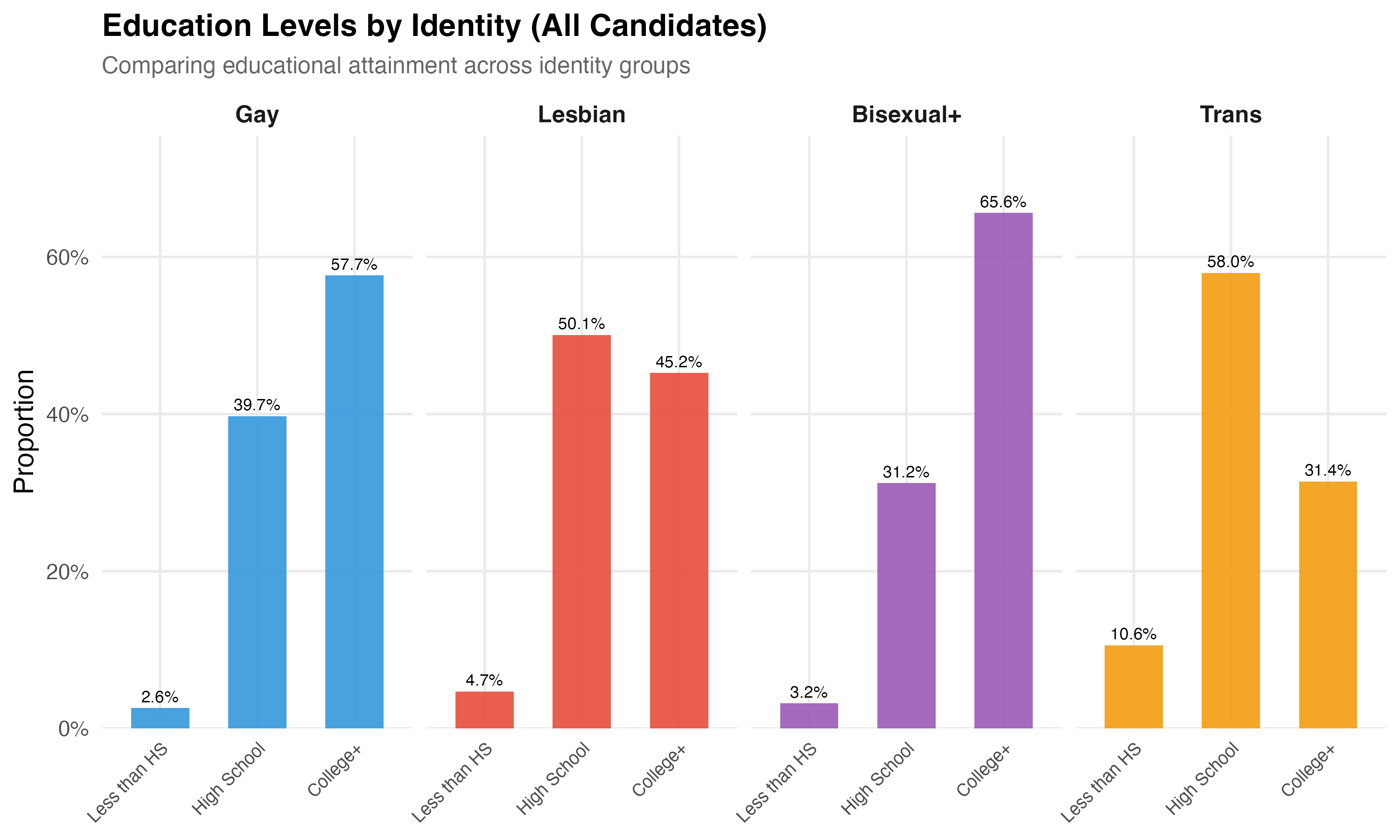
p_edu <- lgbtq_pos %>%
filter(lgbt_category %in% main_categories, !is.na(education_simple)) %>%
mutate(
lgbt_category = factor(lgbt_category, levels = main_categories),
education_simple = factor(education_simple, levels = c("Less than HS", "High School", "College+"))
) %>%
count(lgbt_category, education_simple) %>%
group_by(lgbt_category) %>%
mutate(pct = n / sum(n)) %>%
ungroup() %>%
ggplot(aes(x = education_simple, y = pct, fill = lgbt_category)) +
geom_col(alpha = 0.9, width = 0.6, show.legend = FALSE) +
geom_text(aes(label = format_pct(pct)), vjust = -0.5, size = 3) +
facet_wrap(~lgbt_category, nrow = 1) +
scale_y_continuous(labels = percent, expand = expansion(mult = c(0, 0.15))) +
scale_fill_manual(values = pal_identity) +
labs(
x = NULL, y = "Proportion",
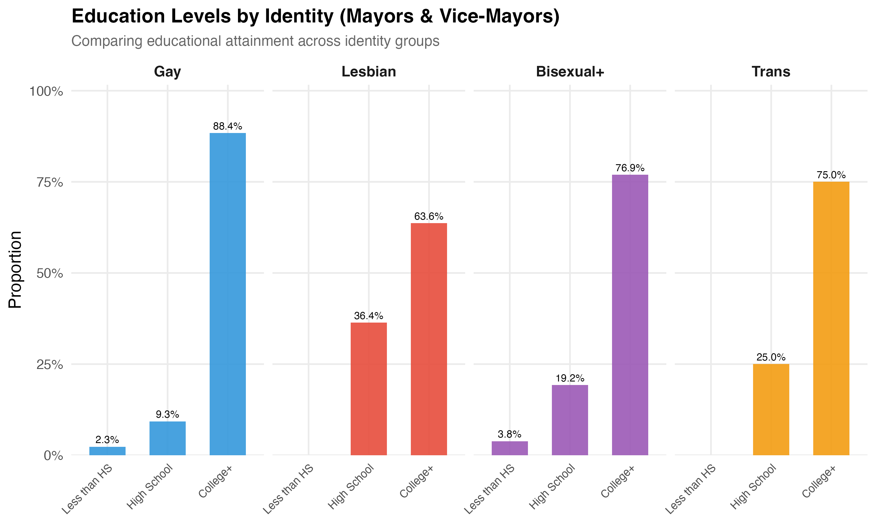
title = paste0("Education Levels by Identity (", tab_name, ")"),
subtitle = "Comparing educational attainment across identity groups"
) +
theme(axis.text.x = element_text(angle = 45, hjust = 1, size = 9))
cat_plot(p_edu, paste0("03-education-by-identity-", pos_suffix(tab_name)), height = 6)
cat("::: {.callout-note}\n")
cat("## Trans Educational Attainment\n")
cat("Brazil's trans population faces well-documented barriers to educational attainment, ",
"including school exclusion, bullying, and economic marginalization. Any differences ",
"in college completion rates between trans and other LGBTQ+ candidates should be ",
"interpreted in this structural context rather than as reflecting individual capacity.\n")
cat(":::\n\n")
}
render_position_tabset(render_demographics_03, df)
```
Several dimensions warrant attention:
- **Gender composition** differs across categories by definition (Gay candidates are male, Lesbian candidates are female) and by social structure (the gender distribution among Trans and Bisexual+ candidates reflects the composition of each group's candidate pool).
- **Age** varies across identities, potentially reflecting different generational patterns of openness and political entry.
- **Education** differences across groups may reflect structural inequalities --- particularly for trans candidates, who face documented barriers to formal education in Brazil.
# Political Profiles {#sec-political}
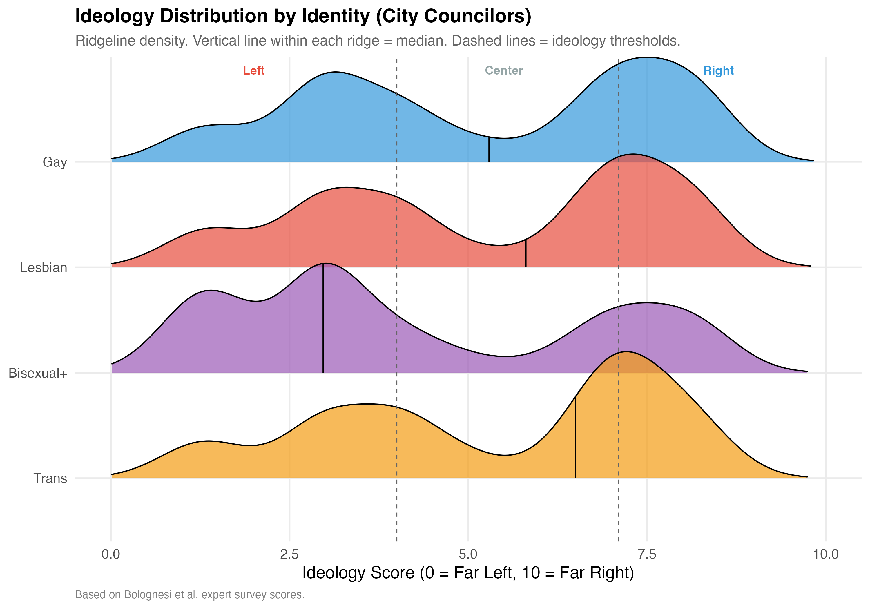
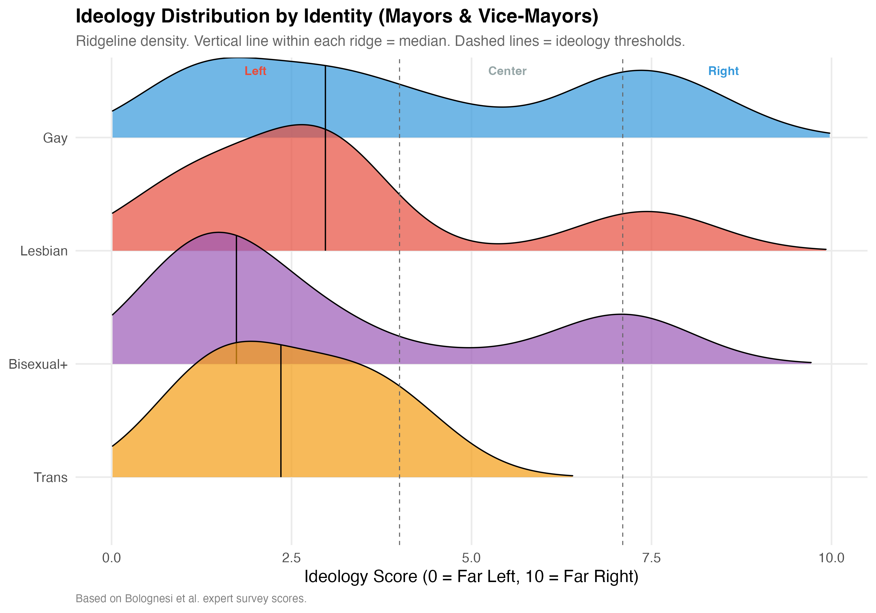
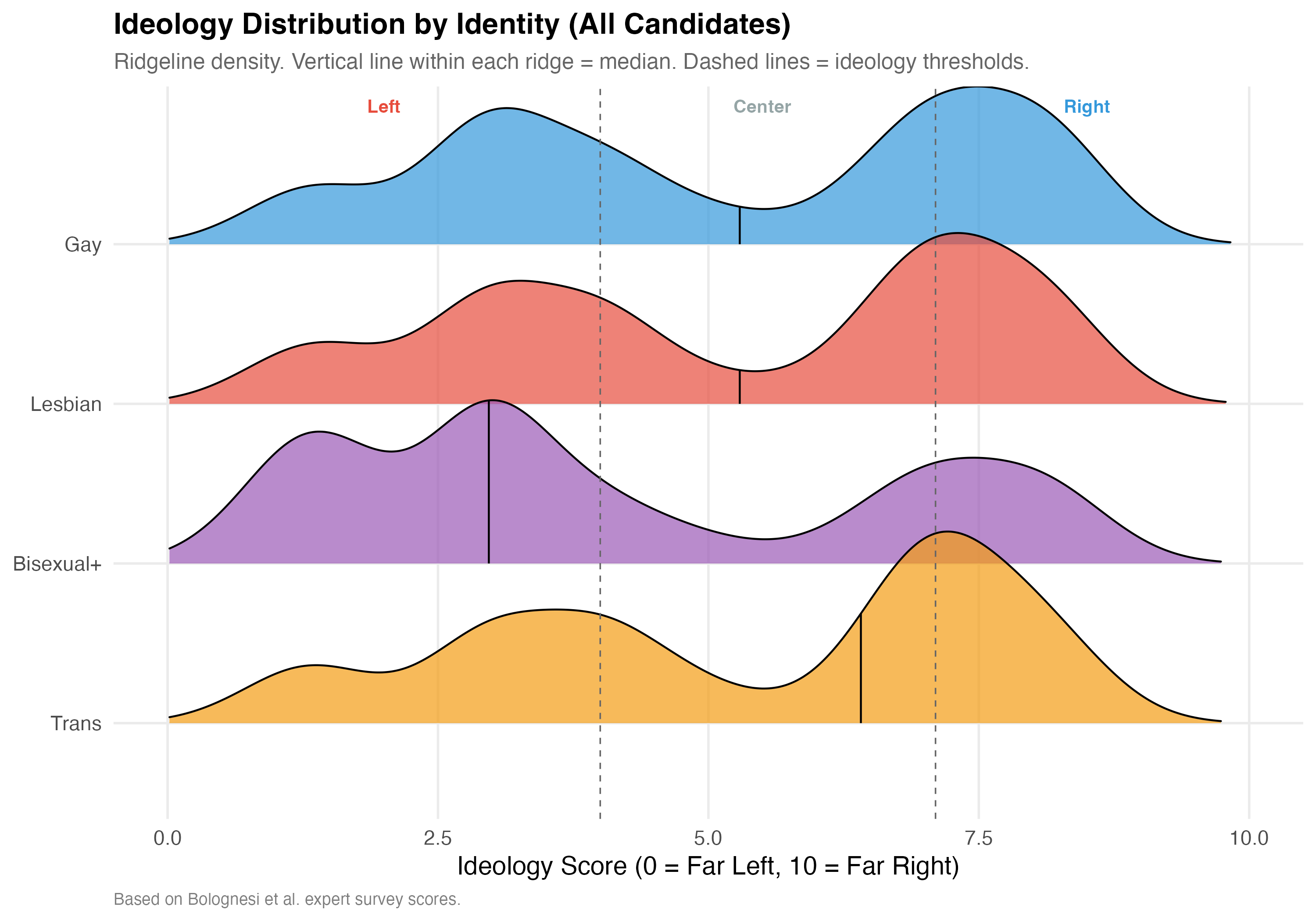
Party ideology scores are drawn from Bolognesi et al.'s expert survey (0--10 left-right scale; Left < 4.0, Center 4.0--7.1, Right > 7.1). The ideological positioning of LGBTQ+ candidates may vary by identity group.
```{r political-tabset}
#| results: asis
render_political_03 <- function(data, tab_name) {
lgbtq_pos <- data %>% filter(lgbtq_candidate)
simplified <- use_simplified(data)
# --- Ideology distribution table ---
cat("### Ideology Distribution\n\n")
ideo_tab <- lgbtq_pos %>%
filter(!is.na(ideology_category), lgbt_category %in% analysis_categories) %>%
count(lgbt_category, ideology_category) %>%
group_by(lgbt_category) %>%
mutate(pct = format_pct(n / sum(n))) %>%
ungroup() %>%
select(-n) %>%
pivot_wider(names_from = ideology_category, values_from = pct, values_fill = "0.0%") %>%
rename(Category = lgbt_category)
cat_kable(ideo_tab, align = c("l", "r", "r", "r"))
# --- Ideology score summary ---
cat("### Ideology Scores\n\n")
score_tab <- lgbtq_pos %>%
filter(!is.na(ideology_score), lgbt_category %in% analysis_categories) %>%
group_by(lgbt_category) %>%
summarise(
N = n(),
Mean = round(mean(ideology_score), 2),
SD = round(sd(ideology_score), 2),
Median = round(median(ideology_score), 2),
.groups = "drop"
) %>%
rename(Category = lgbt_category)
cat_kable(score_tab, align = c("l", "r", "r", "r", "r"))
# --- Ideology plot ---
cat("### Ideology Distribution Plot\n\n")
if (simplified) {
# Small N: grouped bar chart by ideology category
p_ideo <- lgbtq_pos %>%
filter(!is.na(ideology_category), lgbt_category %in% main_categories) %>%
mutate(lgbt_category = factor(lgbt_category, levels = main_categories)) %>%
count(lgbt_category, ideology_category) %>%
group_by(lgbt_category) %>%
mutate(pct = n / sum(n)) %>%
ungroup() %>%
ggplot(aes(x = ideology_category, y = pct, fill = ideology_category)) +
geom_col(alpha = 0.9, width = 0.6) +
geom_text(aes(label = format_pct(pct)), vjust = -0.5, size = 3) +
facet_wrap(~lgbt_category, nrow = 1) +
scale_y_continuous(labels = percent, expand = expansion(mult = c(0, 0.15))) +
scale_fill_manual(values = pal_ideology, guide = "none") +
labs(
x = NULL, y = "Proportion",
title = paste0("Ideology by Identity (", tab_name, ")"),
subtitle = "Bar chart of ideology categories within each identity group",
caption = "Based on Bolognesi et al. expert survey scores."
)
} else {
# Large N: ridgeline density
p_ideo <- lgbtq_pos %>%
filter(!is.na(ideology_score), lgbt_category %in% main_categories) %>%
mutate(lgbt_category = factor(lgbt_category, levels = rev(main_categories))) %>%
ggplot(aes(x = ideology_score, y = lgbt_category, fill = lgbt_category)) +
geom_density_ridges(
alpha = 0.7, scale = 1.2, rel_min_height = 0.01,
quantile_lines = TRUE, quantiles = 2
) +
geom_vline(xintercept = c(4, 7.1), linetype = "dashed", color = "gray40", linewidth = 0.4) +
annotate("text", x = 2, y = Inf, label = "Left", vjust = 2,
color = "#E74C3C", fontface = "bold", size = 3.5) +
annotate("text", x = 5.5, y = Inf, label = "Center", vjust = 2,
color = "#95A5A6", fontface = "bold", size = 3.5) +
annotate("text", x = 8.5, y = Inf, label = "Right", vjust = 2,
color = "#3498DB", fontface = "bold", size = 3.5) +
scale_fill_manual(values = pal_identity, guide = "none") +
scale_x_continuous(limits = c(0, 10)) +
labs(
x = "Ideology Score (0 = Far Left, 10 = Far Right)", y = NULL,
title = paste0("Ideology Distribution by Identity (", tab_name, ")"),
subtitle = "Ridgeline density. Vertical line within each ridge = median. Dashed lines = ideology thresholds.",
caption = "Based on Bolognesi et al. expert survey scores."
)
}
cat_plot(p_ideo, paste0("03-ideology-", pos_suffix(tab_name)), height = 7)
# --- Top parties ---
n_top <- if (simplified) 2 else 3
cat(paste0("### Top ", n_top, " Parties by Identity\n\n"))
top_parties <- lgbtq_pos %>%
filter(lgbt_category %in% analysis_categories) %>%
count(lgbt_category, party_abbrev, sort = TRUE) %>%
group_by(lgbt_category) %>%
mutate(rank = row_number(), pct = format_pct(n / sum(n))) %>%
filter(rank <= n_top) %>%
ungroup() %>%
select(Category = lgbt_category, Rank = rank, Party = party_abbrev,
N = n, `% within Category` = pct)
cat_kable(top_parties, align = c("l", "r", "l", "r", "r"))
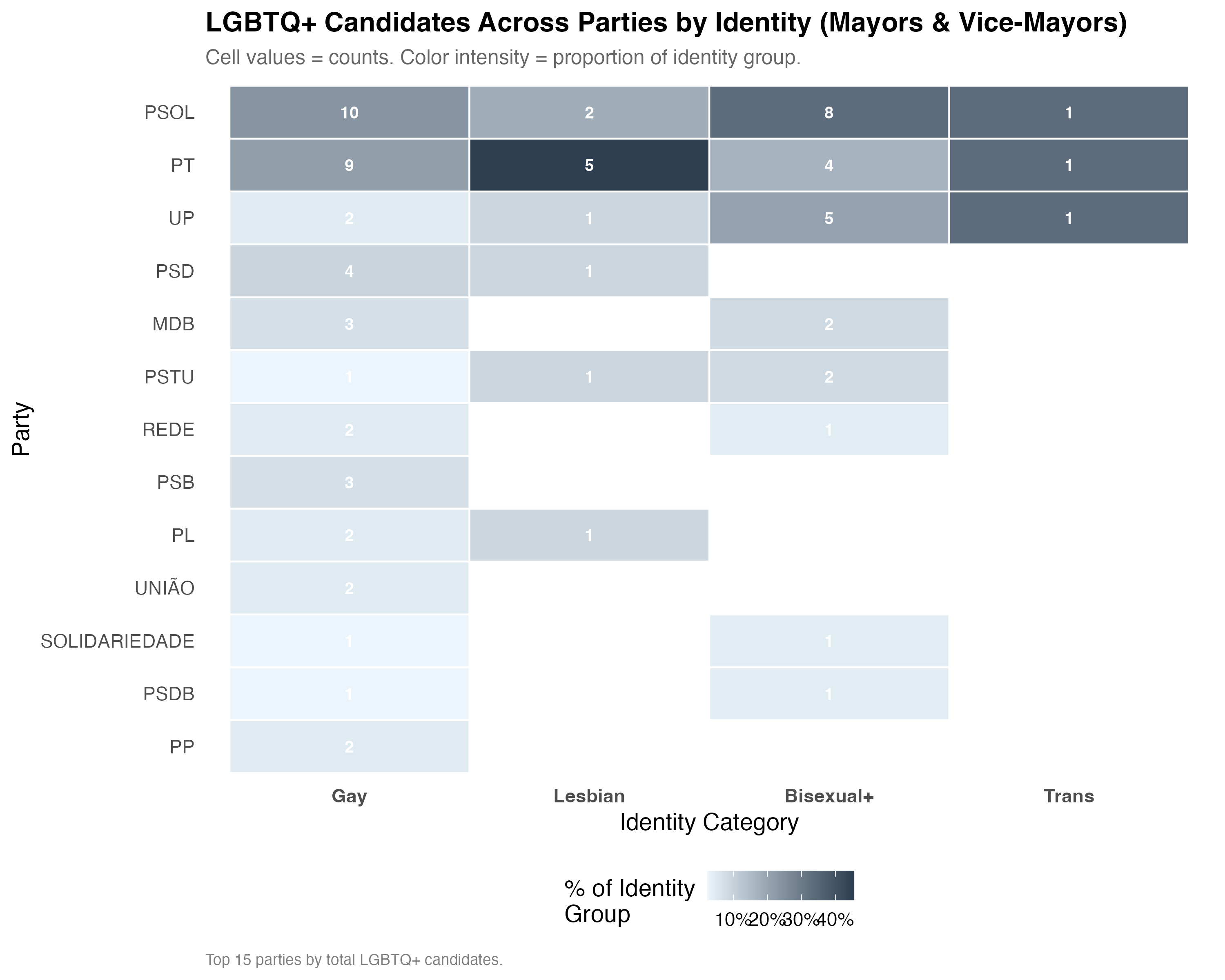
# --- Party-identity heatmap ---
cat("### Party x Identity Heatmap\n\n")
n_parties <- if (simplified) 8 else 15
top_lgbtq_parties <- lgbtq_pos %>%
count(party_abbrev, sort = TRUE) %>%
head(n_parties) %>%
pull(party_abbrev)
heatmap_data <- lgbtq_pos %>%
filter(party_abbrev %in% top_lgbtq_parties, lgbt_category %in% main_categories) %>%
count(party_abbrev, lgbt_category) %>%
group_by(lgbt_category) %>%
mutate(pct = n / sum(n)) %>%
ungroup()
p_heat <- heatmap_data %>%
ggplot(aes(
x = factor(lgbt_category, levels = main_categories),
y = reorder(party_abbrev, n, FUN = sum),
fill = pct
)) +
geom_tile(color = "white", linewidth = 0.5) +
geom_text(aes(label = n), size = 3.5, color = "white", fontface = "bold") +
scale_fill_gradient(
low = "#EBF5FB", high = "#2C3E50",
labels = percent, name = "% of Identity\nGroup"
) +
labs(
x = "Identity Category", y = "Party",
title = paste0("LGBTQ+ Candidates Across Parties by Identity (", tab_name, ")"),
subtitle = "Cell values = counts. Color intensity = proportion of identity group.",
caption = paste0("Top ", n_parties, " parties by total LGBTQ+ candidates.")
) +
theme(
panel.grid = element_blank(),
axis.text.x = element_text(face = "bold")
)
cat_plot(p_heat, paste0("03-party-heatmap-", pos_suffix(tab_name)), height = 8)
cat("::: {.callout-note}\n")
cat("## Party Preferences Differ by Identity\n")
cat("The heatmap reveals the extent to which different identity groups concentrate ",
"in different parties. If party preferences vary across identities, this suggests ",
"that different groups face distinct opportunity structures in the party system. ",
"Parties that are receptive to some LGBTQ+ identities may not be equally receptive to all.\n")
cat(":::\n\n")
}
render_position_tabset(render_political_03, df)
```
# Electoral Outcomes {#sec-outcomes}
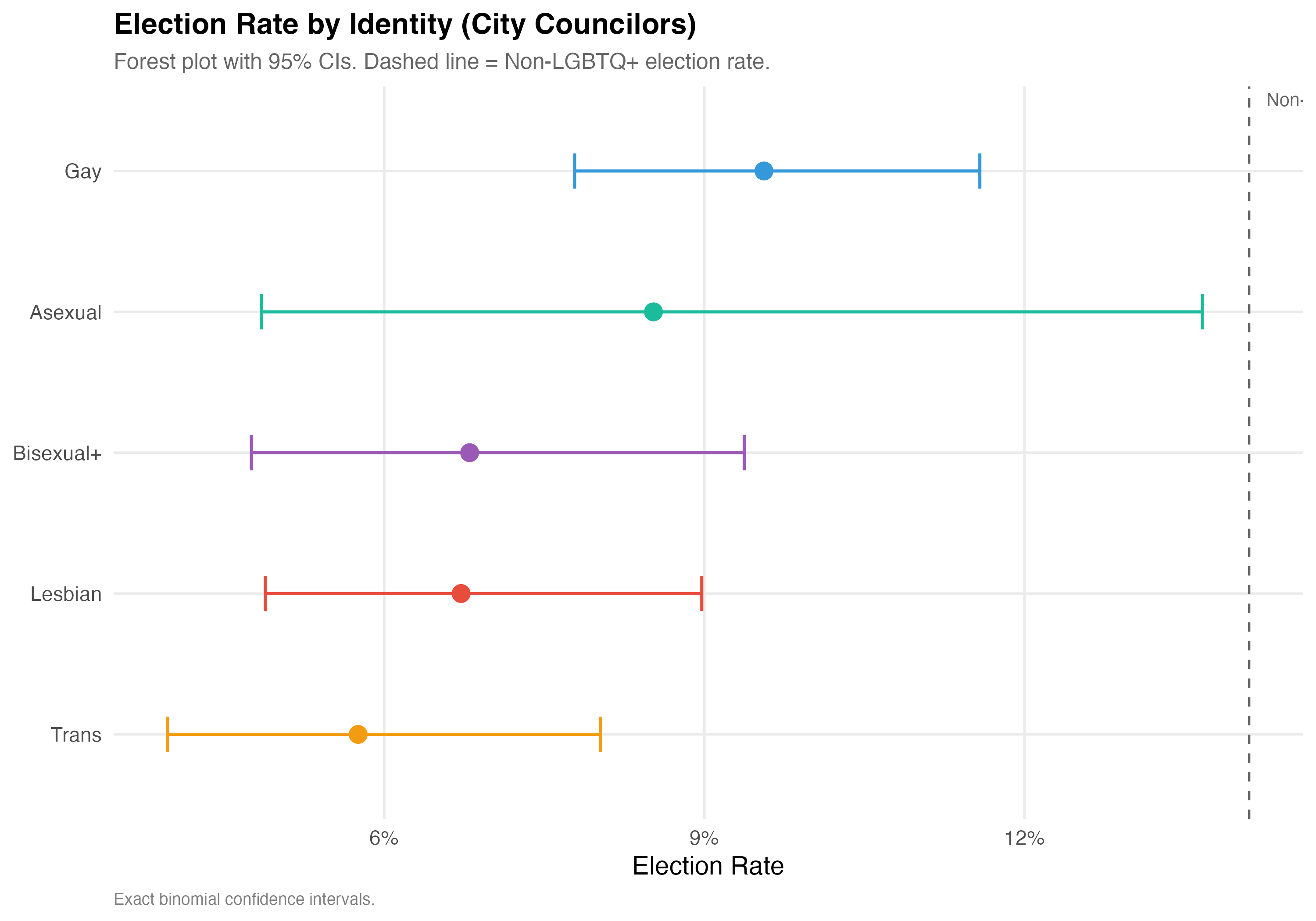
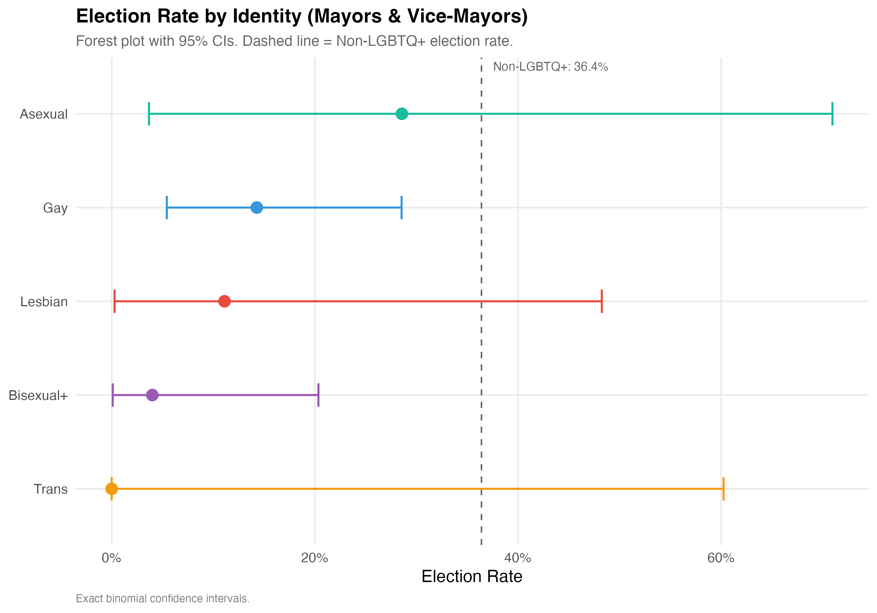
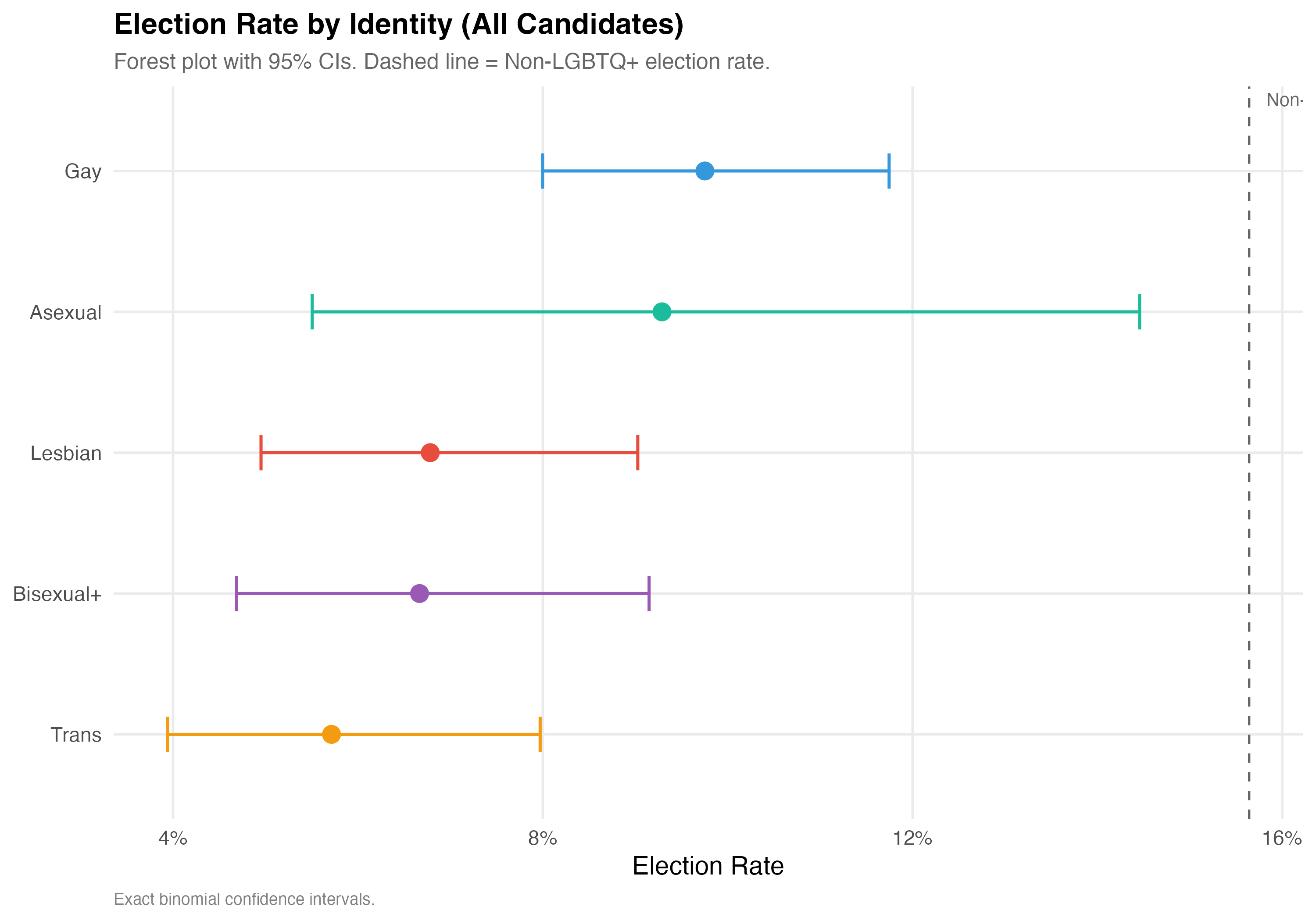
**Election rate** is the proportion of candidates who won their race (elected = 1), including outright winners and those elected by average in proportional races. The panels below report election rates for each identity category, with exact binomial 95% confidence intervals to account for varying sample sizes.
```{r outcomes-tabset}
#| results: asis
render_outcomes_03 <- function(data, tab_name) {
  lgbtq_pos <- data %>% filter(lgbtq_candidate)

  # --- Election rate table ---
  cat("### Election Rates\n\n")

  election_by_id <- lgbtq_pos %>%
    filter(!is.na(elected), lgbt_category %in% analysis_categories) %>%
    group_by(lgbt_category) %>%
    summarise(
      N = n(),
      Elected = sum(elected),
      Rate = mean(elected),
      .groups = "drop"
    ) %>%
    rowwise() %>%
    mutate(
      ci = list(binom.test(Elected, N)$conf.int),
      CI_low = ci[1],
      CI_high = ci[2]
    ) %>%
    ungroup() %>%
    select(-ci)

  election_by_id %>%
    mutate(
      `Election Rate` = format_pct(Rate),
      `95% CI` = paste0("[", format_pct(CI_low), ", ", format_pct(CI_high), "]"),
      N = format_n(N),
      Elected = format_n(Elected)
    ) %>%
    select(Category = lgbt_category, N, Elected, `Election Rate`, `95% CI`) %>%
    cat_kable(align = c("l", "r", "r", "r", "r"))

  # --- Forest plot ---
  cat("### Forest Plot\n\n")

  ref_rate <- data %>%
    filter(!lgbtq_candidate, !is.na(elected)) %>%
    summarise(rate = mean(elected)) %>%
    pull(rate)

  p_forest <- election_by_id %>%
    mutate(
      lgbt_category = fct_reorder(lgbt_category, Rate),
      sig = ifelse(CI_low > ref_rate, "Above",
                   ifelse(CI_high < ref_rate, "Below", "Overlaps"))
    ) %>%
    ggplot(aes(x = Rate, y = lgbt_category, color = lgbt_category)) +
    geom_vline(
      xintercept = ref_rate,
      linetype = "dashed", color = "gray40", linewidth = 0.6
    ) +
    annotate("text", x = ref_rate, y = Inf,
             label = paste0("Non-LGBTQ+: ", format_pct(ref_rate)),
             hjust = -0.1, vjust = 1.5, size = 3.5, color = "gray40") +
    geom_errorbarh(
      aes(xmin = CI_low, xmax = CI_high),
      height = 0.25, linewidth = 0.8
    ) +
    geom_point(size = 4) +
    scale_x_continuous(labels = percent) +
    scale_color_manual(values = pal_identity, guide = "none") +
    labs(
      x = "Election Rate", y = NULL,
      title = paste0("Election Rate by Identity (", tab_name, ")"),
      subtitle = "Forest plot with 95% CIs. Dashed line = Non-LGBTQ+ election rate.",
      caption = "Exact binomial confidence intervals."
    )
  cat_plot(p_forest, paste0("03-forest-election-", pos_suffix(tab_name)), height = 7)

  cat("::: {.callout-note}\n")
  cat("## Small Sample Caveat\n")
  n_asexual <- sum(lgbtq_pos$lgbt_category == "Asexual")
  cat(paste0("The Asexual category in this tab contains ", format_n(n_asexual),
             " candidates. While included for completeness, its estimates carry wider ",
             "confidence intervals than the four main categories --- Gay, Lesbian, ",
             "Bisexual+, and Trans --- which provide the most reliable within-group comparisons.\n"))
  cat(":::\n\n")
}

render_position_tabset(render_outcomes_03, df)
```
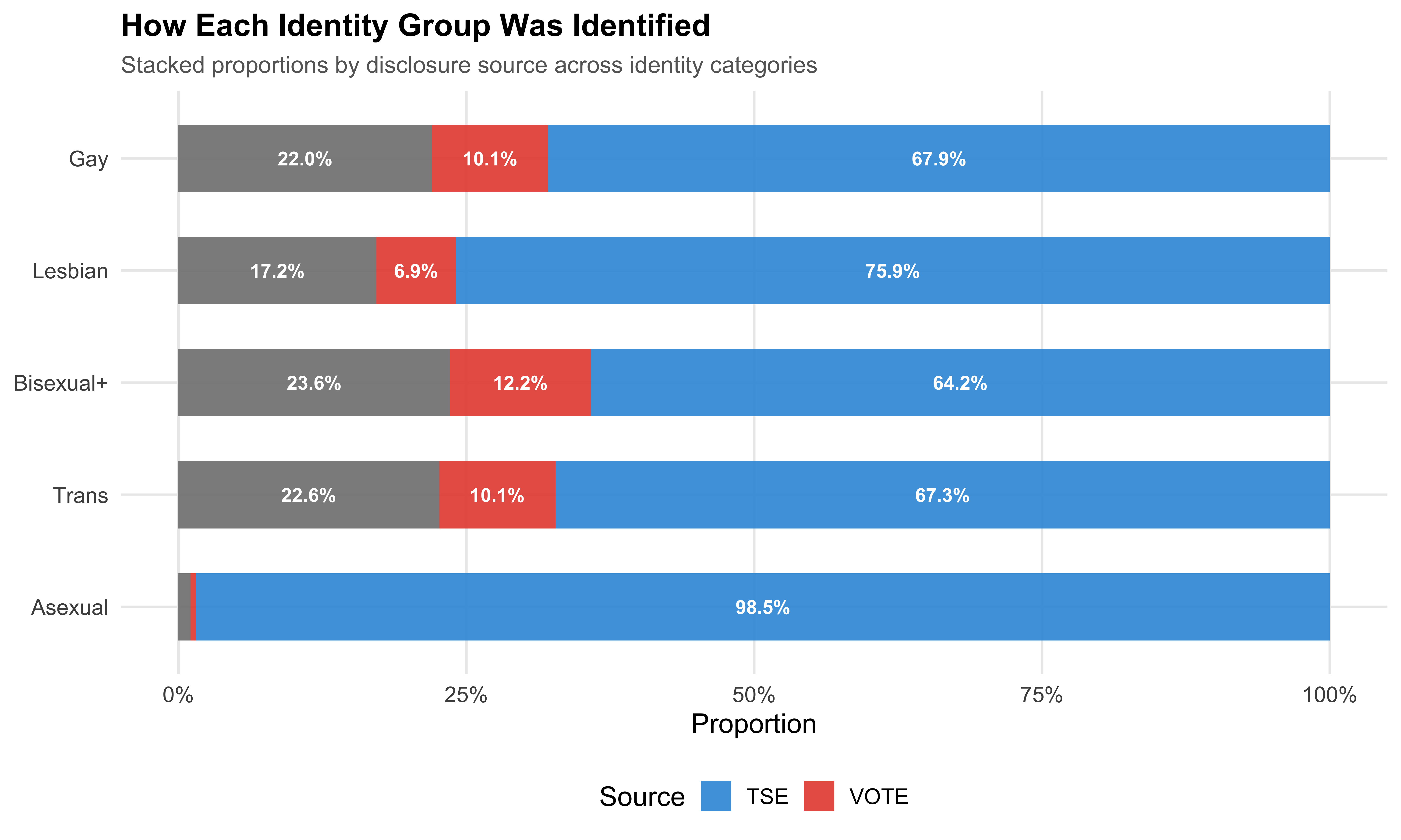
# Disclosure Patterns {#sec-disclosure}
## How Are Different Identities Identified?
**Disclosure source** indicates whether a candidate was identified via TSE self-declaration, VOTE LGBT external matching, or both. The relationship between identity and disclosure source is substantively important: gender identity (trans status) may be more publicly visible --- and therefore more likely to be captured by VOTE LGBT through public campaigning --- whereas sexual orientation may be more private and more often revealed through TSE self-declaration.
::: {.callout-note}
## Pooled Across Positions
Disclosure patterns are presented pooled across city councilors and mayors/vice-mayors. The disclosure source reflects the **identification methodology** (TSE self-declaration vs. VOTE LGBT project) rather than a position-specific outcome. The pathway through which candidates are identified as LGBTQ+ is unlikely to vary systematically by the office sought.
:::
```{r tbl-disclosure-by-identity}
#| label: tbl-disclosure-by-identity
#| tbl-cap: "Identity Category by Disclosure Source"
disclosure_tab <- lgbtq %>%
  filter(lgbt_category %in% analysis_categories) %>%
  count(lgbt_category, disclosure_source) %>%
  group_by(lgbt_category) %>%
  mutate(pct = n / sum(n)) %>%
  ungroup()

# Wide format for table
disclosure_tab %>%
  mutate(cell = paste0(n, " (", format_pct(pct), ")")) %>%
  select(lgbt_category, disclosure_source, cell) %>%
  pivot_wider(names_from = disclosure_source, values_from = cell, values_fill = "0 (0.0%)") %>%
  rename(Category = lgbt_category) %>%
  kable(align = c("l", rep("r", ncol(.) - 1)))
```
```{r fig-disclosure-by-identity}
#| label: fig-disclosure-by-identity
#| fig-cap: "Disclosure Source by Identity Category (Stacked Bars)"
#| fig-height: 6
lgbtq %>%
  filter(lgbt_category %in% analysis_categories) %>%
  count(lgbt_category, disclosure_source) %>%
  group_by(lgbt_category) %>%
  mutate(pct = n / sum(n)) %>%
  ungroup() %>%
  ggplot(aes(x = fct_reorder(lgbt_category, -as.numeric(factor(lgbt_category))),
             y = pct, fill = disclosure_source)) +
  geom_col(alpha = 0.9, width = 0.6) +
  geom_text(
    aes(label = ifelse(pct > 0.05, format_pct(pct), "")),
    position = position_stack(vjust = 0.5), size = 3.5, color = "white", fontface = "bold"
  ) +
  coord_flip() +
  scale_y_continuous(labels = percent) +
  scale_fill_manual(
    values = c("TSE" = "#3498DB", "VOTE" = "#E74C3C", "Both" = "#9B59B6"),
    name = "Source"
  ) +
  labs(
    x = NULL, y = "Proportion",
    title = "How Each Identity Group Was Identified",
    subtitle = "Stacked proportions by disclosure source across identity categories"
  )

save_figure(last_plot(), "03_disclosure_by_identity")
```
# Summary
This chapter demonstrates that "LGBTQ+ candidates" is not a monolithic category. Key takeaways include:
1. **Compositional diversity**: The LGBTQ+ candidate pool comprises several distinct identity categories, each with a different share of the total pool.
2. **Demographic heterogeneity**: Age, gender composition, racial makeup, and educational attainment vary across identity groups, reflecting distinct structural positions within Brazilian society.
3. **Ideological variation**: The degree to which different identity groups concentrate in left, center, or right parties differs. The ridgeline plots reveal distinct distributional shapes rather than a single "LGBTQ+ ideology."
4. **Party sorting**: Different identities concentrate in different parties, suggesting that the party system channels LGBTQ+ representation unevenly.
5. **Electoral outcomes diverge**: Election rates are not uniform across identities. The forest plot and confidence intervals indicate which groups differ from the non-LGBTQ+ baseline.
6. **Disclosure is not random**: The pathway through which candidates are identified as LGBTQ+ (TSE self-declaration vs. VOTE LGBT identification) varies by identity, with implications for data coverage and sample composition.
The next chapter examines the **geographic dimension**: where do LGBTQ+ candidates run, and how does geography interact with the identity patterns documented here?