---
title: "5. Campaign Finance"
subtitle: "Follow the Money: Revenue Sources and Financing Gaps"
---
```{r setup}
source(here::here("code", "00_setup.R"))

# Main analysis data (candidate-level)
df <- readRDS(paths$analysis_full_rds)

# Raw TSE revenue source categories (saved by 02_load_finance_raw.R)
raw_cats <- read_csv(
  paste0(paths$tables, "finance_revenue_source_categories.csv"),
  show_col_types = FALSE
) %>%
  filter(!is.na(DS_ORIGEM_RECEITA))

# Transaction-level finance data (for in-kind analysis)
receitas <- readRDS(paths$finance_trans_rds)
```
```{r inline-computations}
# --- Pre-compute POOLED values for inline narrative text in Summary ---

# Overall stats
n_total       <- nrow(df)
n_zero_rev    <- sum(df$total_revenue == 0)
pct_zero_rev  <- mean(df$total_revenue == 0)
median_rev_all <- median(df$total_revenue)
mean_rev_all   <- mean(df$total_revenue)

# LGBTQ+ vs Non-LGBTQ+ comparison (pooled, for Summary)
lgbtq_stats <- df %>%
  group_by(lgbtq_candidate) %>%
  summarise(
    n          = n(),
    mean_rev   = mean(total_revenue),
    median_rev = median(total_revenue),
    pct_zero   = mean(total_revenue == 0),
    mean_pct_self = mean(pct_self, na.rm = TRUE),
    mean_pct_party = mean(pct_party, na.rm = TRUE),
    mean_pct_individual = mean(pct_individual, na.rm = TRUE),
    mean_pct_crowdfunding = mean(pct_crowdfunding, na.rm = TRUE),
    mean_pct_financial = mean(pct_financial, na.rm = TRUE),
    mean_pct_inkind = mean(pct_inkind, na.rm = TRUE),
    .groups = "drop"
  )

lgbtq_median   <- lgbtq_stats$median_rev[lgbtq_stats$lgbtq_candidate == TRUE]
nonlgbtq_median <- lgbtq_stats$median_rev[lgbtq_stats$lgbtq_candidate == FALSE]
lgbtq_mean     <- lgbtq_stats$mean_rev[lgbtq_stats$lgbtq_candidate == TRUE]
nonlgbtq_mean  <- lgbtq_stats$mean_rev[lgbtq_stats$lgbtq_candidate == FALSE]

median_ratio_overall <- lgbtq_median / nonlgbtq_median
mean_ratio_overall   <- lgbtq_mean / nonlgbtq_mean

# Direction labels for inline use
median_direction <- if (lgbtq_median > nonlgbtq_median) "higher" else if (lgbtq_median < nonlgbtq_median) "lower" else "equal"
mean_direction   <- if (lgbtq_mean > nonlgbtq_mean) "higher" else if (lgbtq_mean < nonlgbtq_mean) "lower" else "equal"

# LGBTQ+ funding composition
lgbtq_pct_party      <- lgbtq_stats$mean_pct_party[lgbtq_stats$lgbtq_candidate == TRUE]
nonlgbtq_pct_party   <- lgbtq_stats$mean_pct_party[lgbtq_stats$lgbtq_candidate == FALSE]
lgbtq_pct_individual <- lgbtq_stats$mean_pct_individual[lgbtq_stats$lgbtq_candidate == TRUE]
nonlgbtq_pct_individual <- lgbtq_stats$mean_pct_individual[lgbtq_stats$lgbtq_candidate == FALSE]
lgbtq_pct_self       <- lgbtq_stats$mean_pct_self[lgbtq_stats$lgbtq_candidate == TRUE]
nonlgbtq_pct_self    <- lgbtq_stats$mean_pct_self[lgbtq_stats$lgbtq_candidate == FALSE]

# Identity category stats (pooled, for Summary)
identity_stats <- df %>%
  filter(lgbtq_candidate, lgbt_category != "Other LGBTQ+") %>%
  group_by(lgbt_category) %>%
  summarise(
    mean_pct_party = mean(pct_party, na.rm = TRUE),
    mean_pct_individual = mean(pct_individual, na.rm = TRUE),
    median_rev = median(total_revenue),
    .groups = "drop"
  )

# Find which category has the highest party share
top_party_cat <- identity_stats %>% slice_max(mean_pct_party, n = 1) %>% pull(lgbt_category)
top_party_val <- identity_stats %>% slice_max(mean_pct_party, n = 1) %>% pull(mean_pct_party)
top_indiv_cat <- identity_stats %>% slice_max(mean_pct_individual, n = 1) %>% pull(lgbt_category)
top_indiv_val <- identity_stats %>% slice_max(mean_pct_individual, n = 1) %>% pull(mean_pct_individual)
```
# Overview
Campaign finance is the lifeblood of electoral competition. In Brazil's municipal elections, candidates must register all revenue with the *Tribunal Superior Eleitoral* (TSE), creating a comprehensive public record of who funds whom. This chapter provides a transparent, ground-up analysis of campaign revenue --- from raw source categories through aggregate patterns --- with special attention to how LGBTQ+ candidates' financial profiles differ from the broader candidate population.
We proceed in four stages: (1) documenting the raw data categories for full transparency, (2) describing general revenue patterns across all candidates, (3) comparing LGBTQ+ and non-LGBTQ+ financing, and (4) disaggregating by identity category and party.
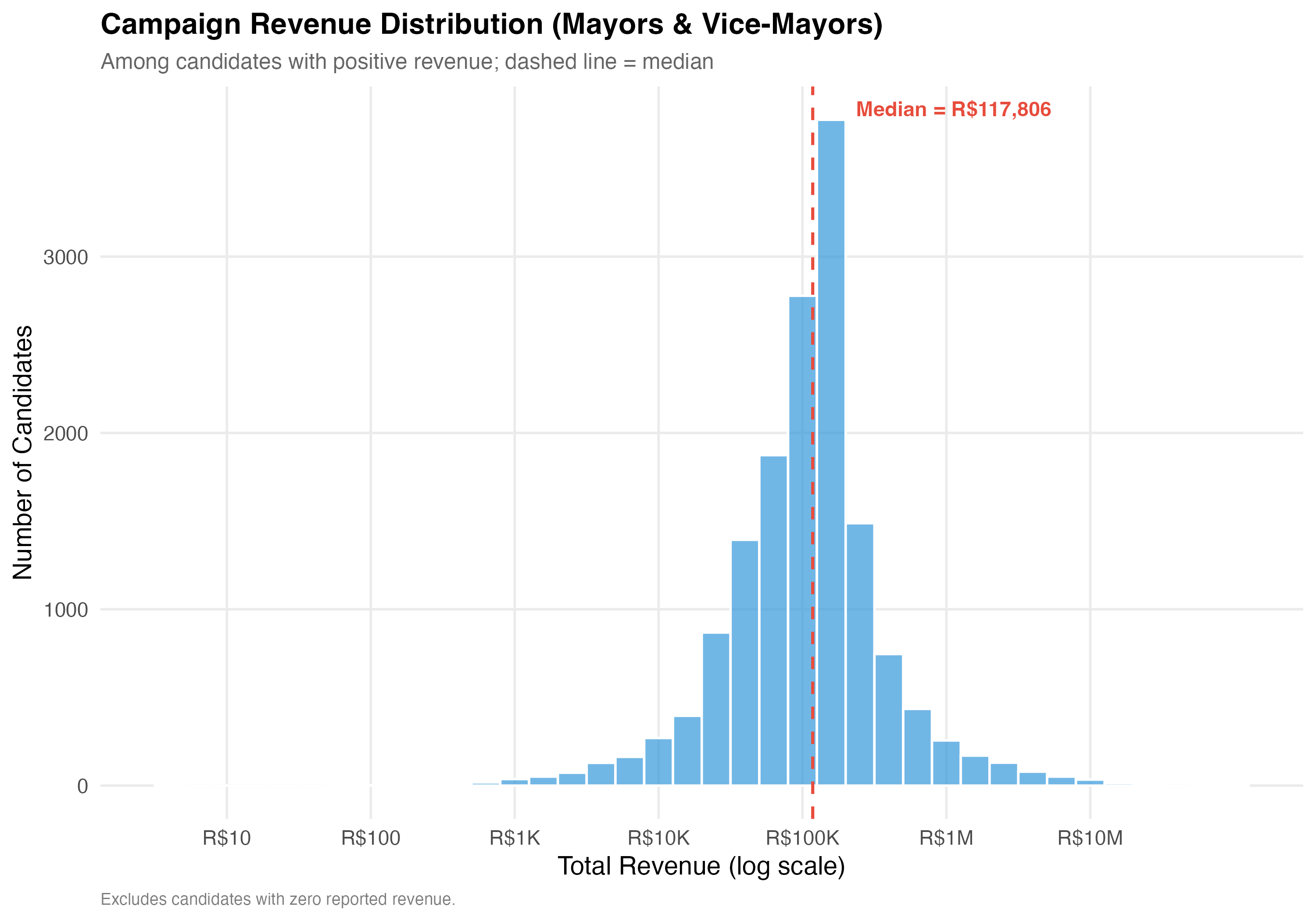
::: {.callout-note}
## Results by Position Type
Campaign revenue differs **dramatically** by position: city councilor campaigns are typically an order of magnitude smaller than mayoral campaigns. To avoid conflating these fundamentally different scales, the main comparison sections are presented separately for **city councilors** and **mayors/vice-mayors** using tabbed panels.
:::
# Raw Data Documentation
## TSE Revenue Source Categories
The TSE raw finance file classifies each transaction by `DS_ORIGEM_RECEITA` (revenue source). Before any analysis, we display the complete frequency table of these raw categories, along with our classification scheme. This is the foundation of all subsequent finance analysis.
```{r tbl-raw-categories}
#| label: tbl-raw-categories
#| tbl-cap: "Complete TSE Revenue Source Categories with Classification"
# Add the classification mapping used in 02_load_finance_raw.R
raw_cats <- raw_cats %>%
  mutate(
    classification = case_when(
      str_detect(DS_ORIGEM_RECEITA, "(?i)recursos pr")           ~ "Self-funding",
      str_detect(DS_ORIGEM_RECEITA, "(?i)partido pol")           ~ "Party funding",
      str_detect(DS_ORIGEM_RECEITA, "(?i)pessoas f")             ~ "Individual donation",
      str_detect(DS_ORIGEM_RECEITA, "(?i)financiamento coletivo") ~ "Crowdfunding",
      str_detect(DS_ORIGEM_RECEITA, "(?i)outros candidatos")     ~ "Other candidates",
      str_detect(DS_ORIGEM_RECEITA, "(?i)internet")              ~ "Online donations",
      str_detect(DS_ORIGEM_RECEITA, "#NULO")                     ~ "Null/Unclassified",
      TRUE                                                       ~ "Other"
    ),
    total_brl     = replace_na(total_brl, 0),
    total_brl_fmt = format_brl(total_brl),
    pct_fmt       = replace_na(pct, "0.0%"),
    n             = replace_na(n, 0L)
  )

raw_cats %>%
  select(
    `TSE Category`    = DS_ORIGEM_RECEITA,
    `N Transactions`  = n,
    `% of Trans.`     = pct_fmt,
    `Total (R$)`      = total_brl_fmt,
    `Our Label`       = classification
  ) %>%
  kable(align = c("l", "r", "r", "r", "l"))
```
::: {.callout-note}
## Transparency Principle
Every transaction in the TSE receitas file is classified using the mapping above. The raw Portuguese-language category names are preserved alongside our English labels so that any researcher can verify the mapping. The classification code is in `code/02_load_finance_raw.R`.
:::
# General Revenue Patterns
## Overall Revenue Distribution
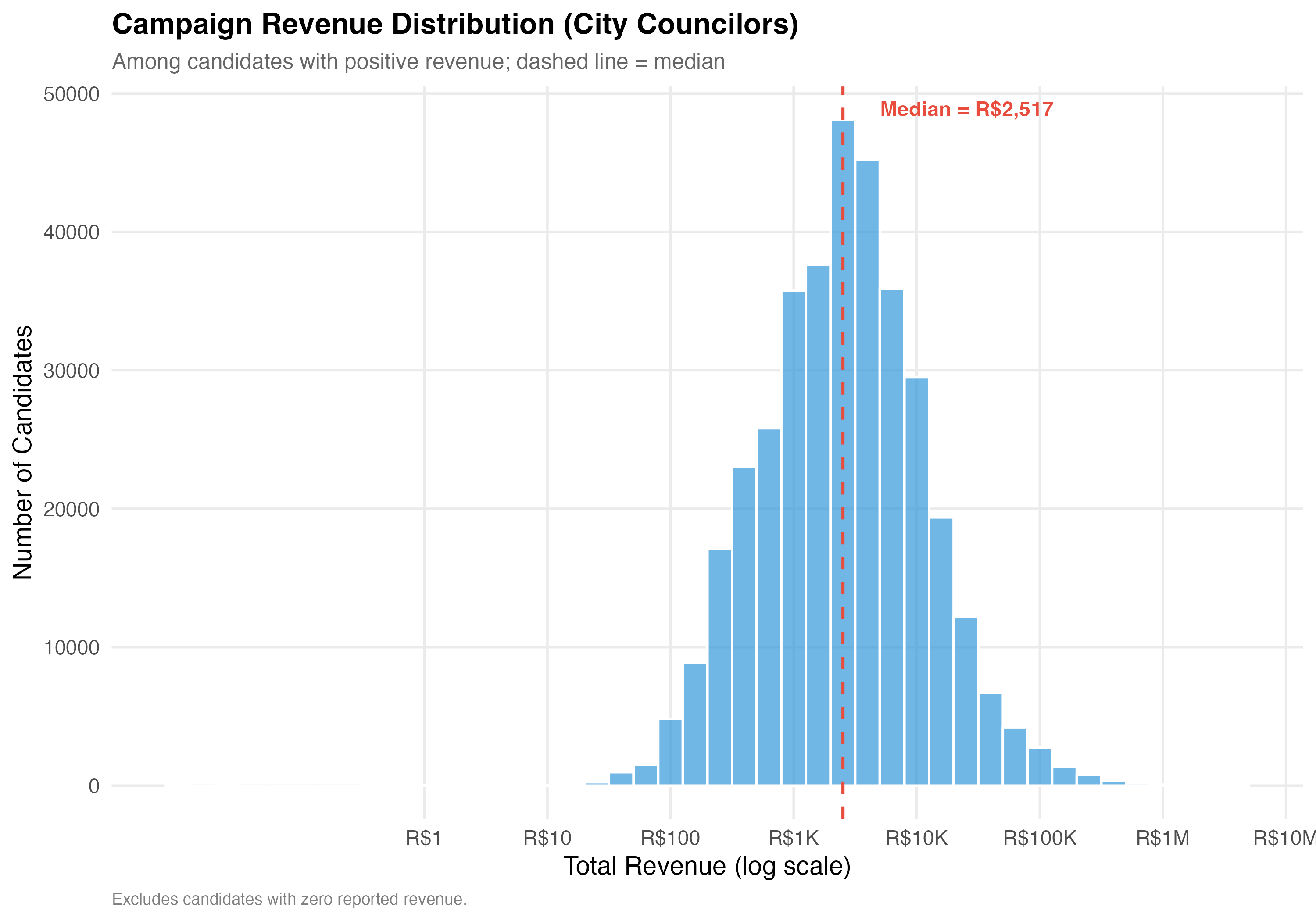
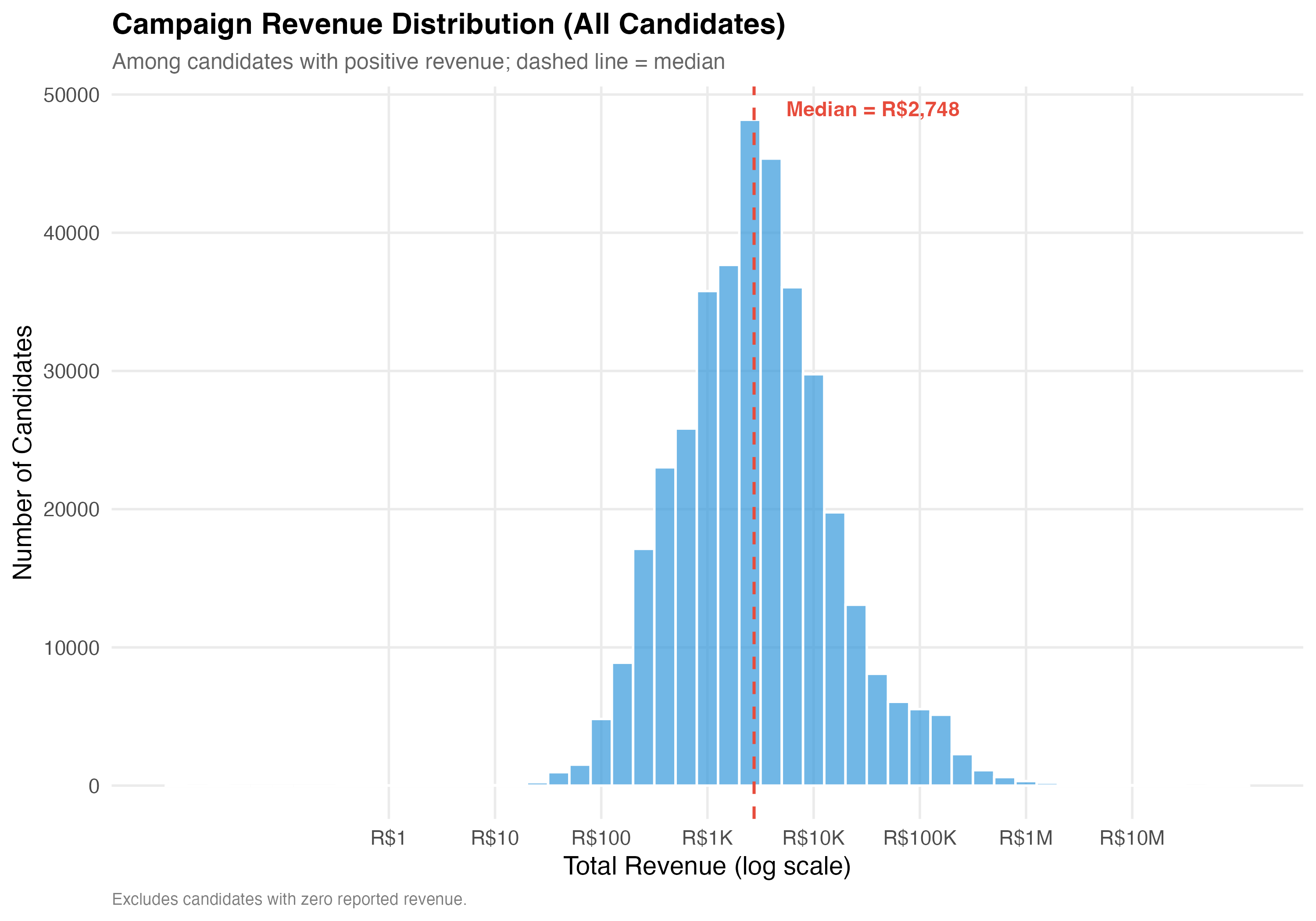
The measure `total_revenue` captures the sum of all campaign receipts registered with the TSE for each candidate, denominated in Brazilian reais (R\$). This includes financial contributions (cash, PIX, bank transfers) and in-kind/estimated contributions (goods and services assigned a monetary value). A candidate with zero total revenue either received no contributions or did not report any.
```{r general-revenue-tabset}
#| results: asis
render_general_revenue <- function(data, tab_name) {
# --- Revenue summary statistics ---
cat("### Revenue Summary Statistics\n\n")
revenue_stats <- data %>%
summarise(
N = format_n(n()),
`Zero Revenue` = format_n(sum(total_revenue == 0)),
`% Zero` = format_pct(mean(total_revenue == 0)),
Mean = format_brl(mean(total_revenue)),
SD = format_brl(sd(total_revenue)),
Median = format_brl(median(total_revenue)),
P25 = format_brl(quantile(total_revenue, 0.25)),
P75 = format_brl(quantile(total_revenue, 0.75)),
P99 = format_brl(quantile(total_revenue, 0.99)),
Max = format_brl(max(total_revenue))
)
revenue_stats %>%
pivot_longer(everything(), names_to = "Statistic", values_to = "Value") %>%
cat_kable(align = c("l", "r"))
# --- Revenue distribution histogram ---
cat("### Revenue Distribution (Log Scale)\n\n")
pos_rev <- data %>% filter(total_revenue > 0)
if (nrow(pos_rev) > 0) {
med_val <- median(pos_rev$total_revenue)
p_dist <- pos_rev %>%
ggplot(aes(x = log10(total_revenue))) +
geom_histogram(binwidth = 0.2, fill = "#3498DB", alpha = 0.7, color = "white") +
geom_vline(xintercept = log10(med_val),
linetype = "dashed", color = "#E74C3C", linewidth = 0.8) +
annotate("text",
x = log10(med_val) + 0.3, y = Inf, vjust = 2, hjust = 0,
label = paste0("Median = ", format_brl(med_val)),
color = "#E74C3C", fontface = "bold", size = 4) +
scale_x_continuous(
breaks = 0:7,
labels = c("R$1", "R$10", "R$100", "R$1K", "R$10K", "R$100K", "R$1M", "R$10M")
) +
labs(
x = "Total Revenue (log scale)",
y = "Number of Candidates",
title = paste0("Campaign Revenue Distribution (", tab_name, ")"),
subtitle = "Among candidates with positive revenue; dashed line = median",
caption = "Excludes candidates with zero reported revenue."
)
cat_plot(p_dist, paste0("05-revenue-dist-", pos_suffix(tab_name)))
}
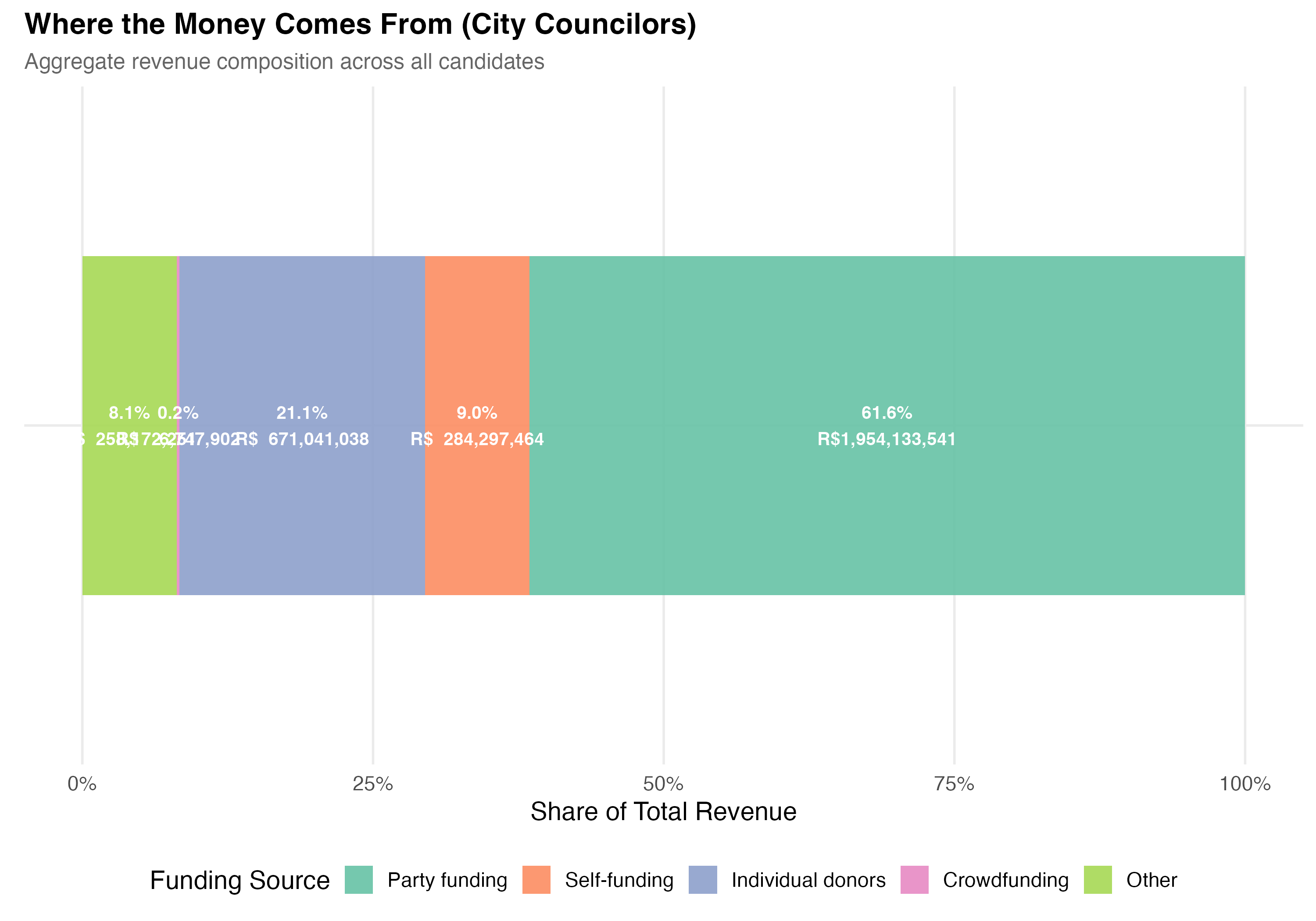
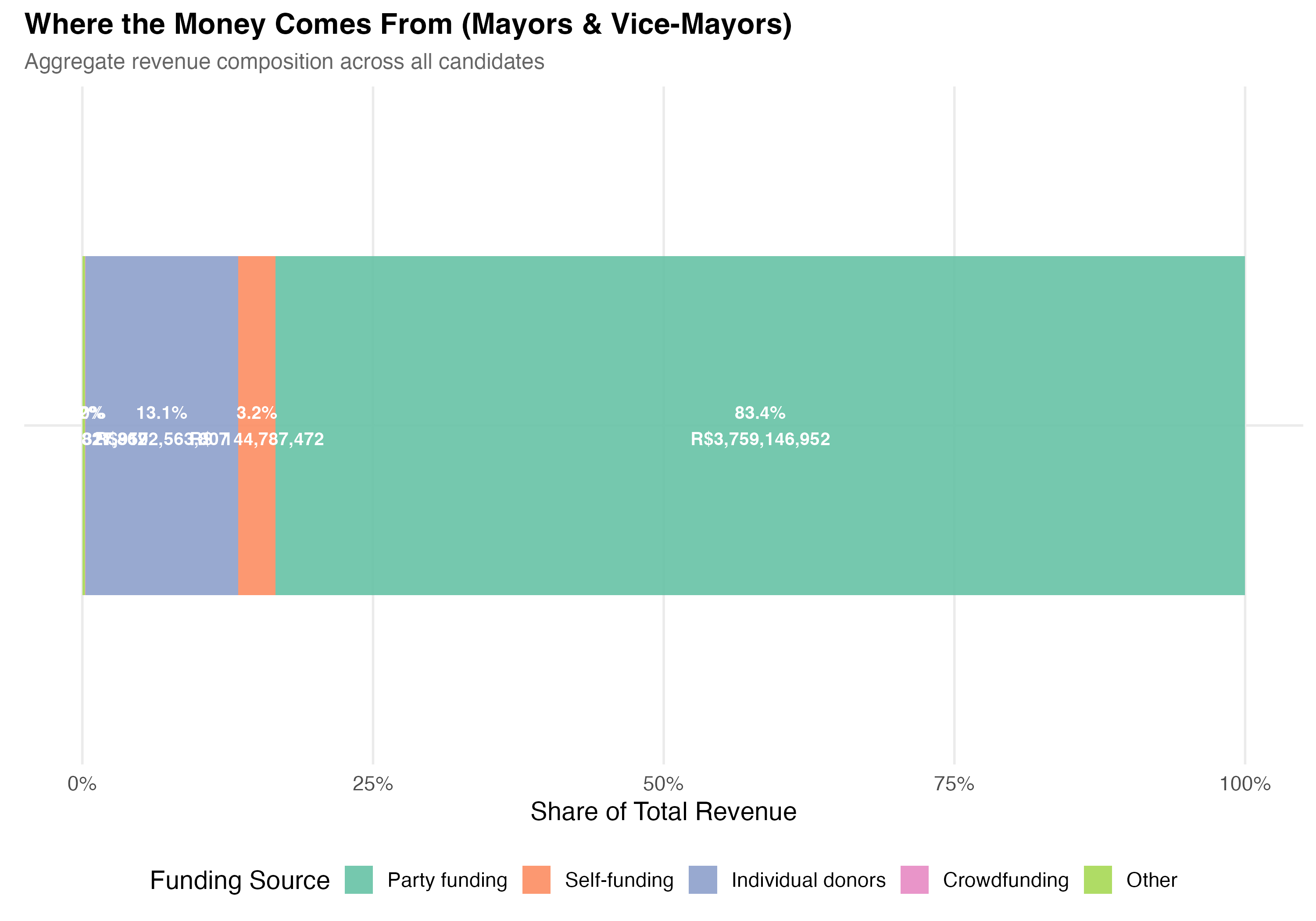
# --- Revenue composition ---
cat("### Revenue Composition by Source\n\n")
comp <- data %>%
summarise(
`Self-funding` = sum(self_funding_amt, na.rm = TRUE),
`Party funding` = sum(party_funding_amt, na.rm = TRUE),
`Individual donors` = sum(individual_funding_amt, na.rm = TRUE),
`Crowdfunding` = sum(crowdfunding_amt, na.rm = TRUE),
`Other` = sum(total_revenue, na.rm = TRUE) -
sum(self_funding_amt, na.rm = TRUE) -
sum(party_funding_amt, na.rm = TRUE) -
sum(individual_funding_amt, na.rm = TRUE) -
sum(crowdfunding_amt, na.rm = TRUE)
) %>%
pivot_longer(everything(), names_to = "source", values_to = "total") %>%
mutate(
pct = total / sum(total),
source = factor(source,
levels = c("Party funding", "Self-funding", "Individual donors",
"Crowdfunding", "Other"))
)
p_comp <- ggplot(comp, aes(x = "", y = pct, fill = source)) +
geom_col(width = 0.6, alpha = 0.9) +
geom_text(aes(label = paste0(format_pct(pct), "\n", format_brl(total))),
position = position_stack(vjust = 0.5), size = 3.5, color = "white",
fontface = "bold") +
coord_flip() +
scale_fill_brewer(palette = "Set2", name = "Funding Source") +
scale_y_continuous(labels = percent) +
labs(
x = NULL,
y = "Share of Total Revenue",
title = paste0("Where the Money Comes From (", tab_name, ")"),
subtitle = "Aggregate revenue composition across all candidates"
)
cat_plot(p_comp, paste0("05-composition-overall-", pos_suffix(tab_name)))
}
render_position_tabset(render_general_revenue, df)
```
# LGBTQ+ vs Non-LGBTQ+ Revenue
```{r lgbtq-revenue-tabset}
#| results: asis
render_lgbtq_revenue <- function(data, tab_name) {
# --- Side-by-side comparison table ---
cat("### Revenue Comparison\n\n")
revenue_comparison <- data %>%
mutate(group = if_else(lgbtq_candidate, "LGBTQ+", "Non-LGBTQ+")) %>%
group_by(group) %>%
summarise(
N = format_n(n()),
`% Zero Rev.` = format_pct(mean(total_revenue == 0)),
`Mean Rev.` = format_brl(mean(total_revenue)),
`Median Rev.` = format_brl(median(total_revenue)),
`SD Rev.` = format_brl(sd(total_revenue)),
`Mean Trans.` = as.character(round(mean(n_transactions), 1)),
`Mean Donors` = as.character(round(mean(n_unique_donors), 1)),
`% Self-fund` = format_pct100(mean(pct_self)),
`% Party` = format_pct100(mean(pct_party)),
`% Individual` = format_pct100(mean(pct_individual)),
`% Crowdfund` = format_pct100(mean(pct_crowdfunding)),
.groups = "drop"
)
revenue_comparison %>%
pivot_longer(-group, names_to = "Metric", values_to = "value") %>%
pivot_wider(names_from = group, values_from = value) %>%
cat_kable(align = c("l", "r", "r"))
# Compute position-specific stats for callout
pos_stats <- data %>%
group_by(lgbtq_candidate) %>%
summarise(
median_rev = median(total_revenue),
mean_rev = mean(total_revenue),
.groups = "drop"
)
lgbtq_med <- pos_stats$median_rev[pos_stats$lgbtq_candidate == TRUE]
non_med <- pos_stats$median_rev[pos_stats$lgbtq_candidate == FALSE]
lgbtq_mn <- pos_stats$mean_rev[pos_stats$lgbtq_candidate == TRUE]
non_mn <- pos_stats$mean_rev[pos_stats$lgbtq_candidate == FALSE]
med_ratio <- if (non_med > 0) lgbtq_med / non_med else NA_real_
mn_ratio <- if (non_mn > 0) lgbtq_mn / non_mn else NA_real_
cat("::: {.callout-note}\n")
cat("## Revenue Comparison\n")
cat(sprintf("In this tab (%s), the median revenue for LGBTQ+ candidates is %s vs. %s for non-LGBTQ+ (ratio: %.2f). ",
tab_name, format_brl(lgbtq_med), format_brl(non_med),
if (!is.na(med_ratio)) med_ratio else 0))
cat(sprintf("At the mean: %s vs. %s (ratio: %.2f).\n",
format_brl(lgbtq_mn), format_brl(non_mn),
if (!is.na(mn_ratio)) mn_ratio else 0))
cat(":::\n\n")
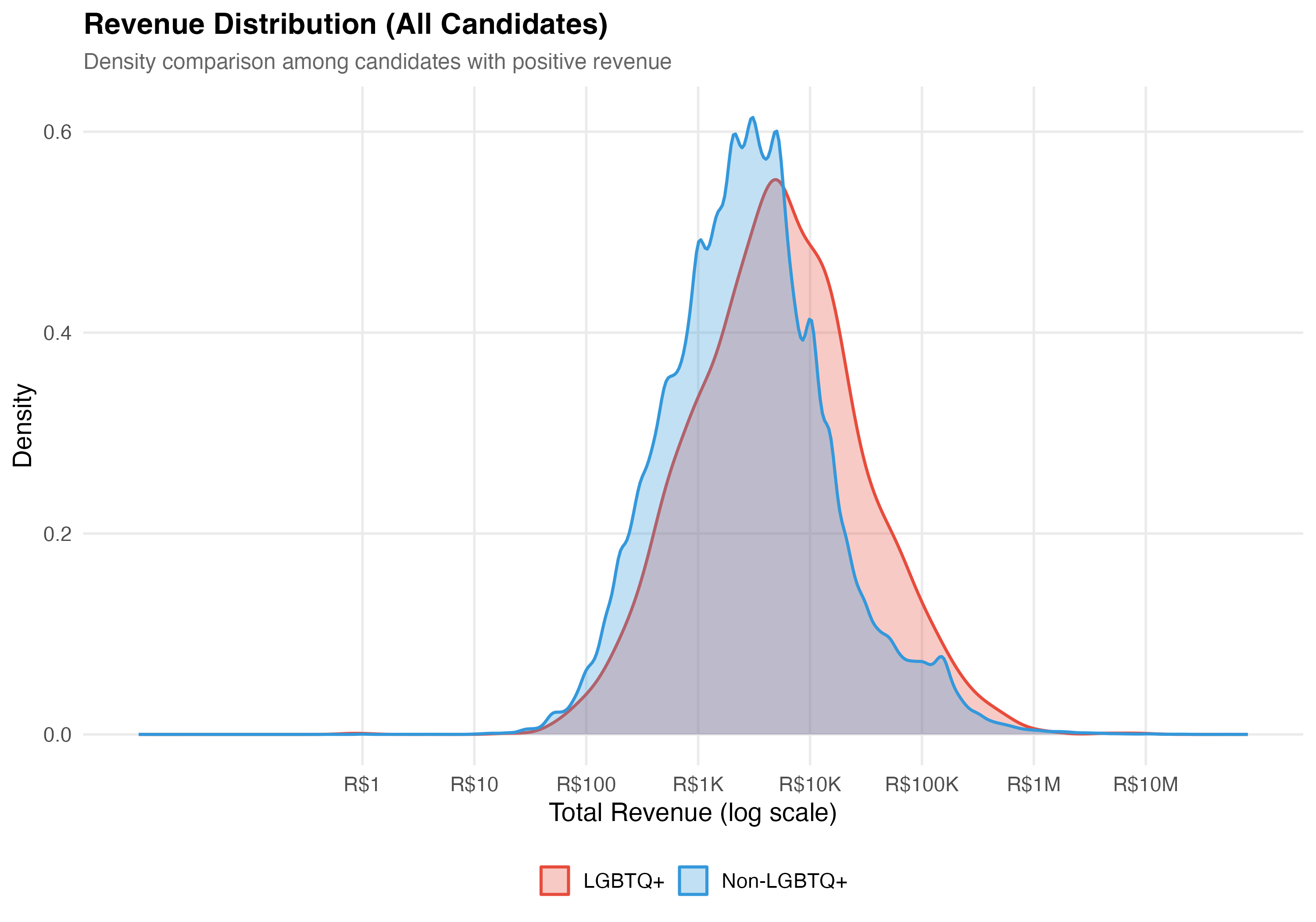
# --- Revenue distribution comparison ---
cat("### Revenue Distribution\n\n")
pos_rev <- data %>% filter(total_revenue > 0)
if (nrow(pos_rev) > 0) {
p_density <- pos_rev %>%
mutate(group = if_else(lgbtq_candidate, "LGBTQ+", "Non-LGBTQ+")) %>%
ggplot(aes(x = log10(total_revenue), fill = group, color = group)) +
geom_density(alpha = 0.3, linewidth = 0.8) +
scale_fill_manual(values = pal_lgbtq, name = NULL) +
scale_color_manual(values = pal_lgbtq, name = NULL) +
scale_x_continuous(
breaks = 0:7,
labels = c("R$1", "R$10", "R$100", "R$1K", "R$10K", "R$100K", "R$1M", "R$10M")
) +
labs(
x = "Total Revenue (log scale)",
y = "Density",
title = paste0("Revenue Distribution (", tab_name, ")"),
subtitle = "Density comparison among candidates with positive revenue"
)
cat_plot(p_density, paste0("05-density-revenue-", pos_suffix(tab_name)))
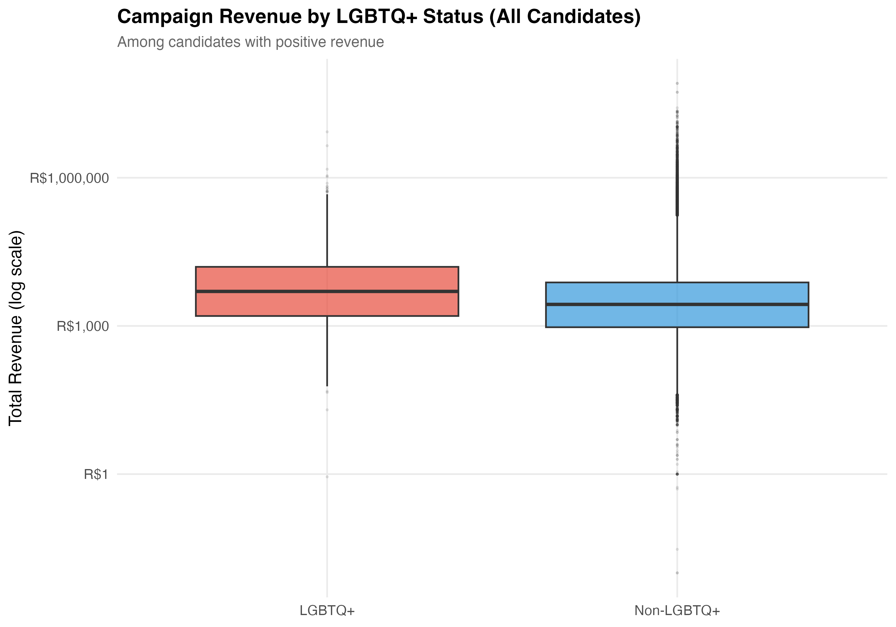
# Box plot
p_box <- pos_rev %>%
mutate(group = if_else(lgbtq_candidate, "LGBTQ+", "Non-LGBTQ+")) %>%
ggplot(aes(x = group, y = total_revenue, fill = group)) +
geom_boxplot(alpha = 0.7, outlier.alpha = 0.1, outlier.size = 0.5) +
scale_y_log10(labels = label_dollar(prefix = "R$", big.mark = ",")) +
scale_fill_manual(values = pal_lgbtq, guide = "none") +
labs(
x = NULL,
y = "Total Revenue (log scale)",
title = paste0("Campaign Revenue by LGBTQ+ Status (", tab_name, ")"),
subtitle = "Among candidates with positive revenue"
)
cat_plot(p_box, paste0("05-box-revenue-", pos_suffix(tab_name)))
}
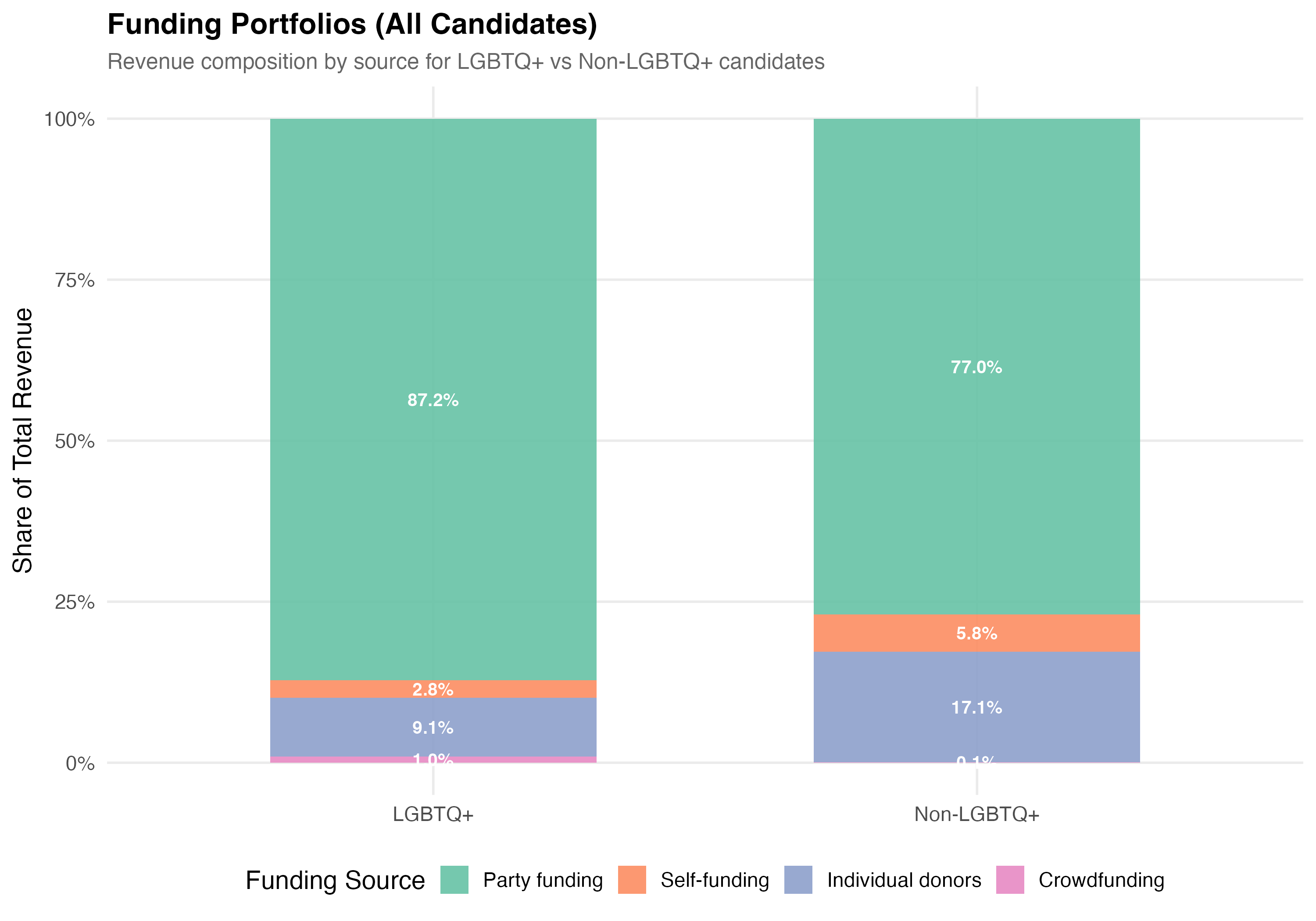
# --- Funding composition ---
cat("### Funding Source Composition\n\n")
p_comp <- data %>%
mutate(group = if_else(lgbtq_candidate, "LGBTQ+", "Non-LGBTQ+")) %>%
group_by(group) %>%
summarise(
`Self-funding` = sum(self_funding_amt, na.rm = TRUE),
`Party funding` = sum(party_funding_amt, na.rm = TRUE),
`Individual donors` = sum(individual_funding_amt, na.rm = TRUE),
`Crowdfunding` = sum(crowdfunding_amt, na.rm = TRUE),
.groups = "drop"
) %>%
pivot_longer(-group, names_to = "source", values_to = "total") %>%
group_by(group) %>%
mutate(pct = total / sum(total)) %>%
ungroup() %>%
mutate(source = factor(source,
levels = c("Party funding", "Self-funding",
"Individual donors", "Crowdfunding"))) %>%
ggplot(aes(x = group, y = pct, fill = source)) +
geom_col(alpha = 0.9, width = 0.6) +
geom_text(aes(label = format_pct(pct)),
position = position_stack(vjust = 0.5), size = 3.5, color = "white",
fontface = "bold") +
scale_fill_brewer(palette = "Set2", name = "Funding Source") +
scale_y_continuous(labels = percent) +
labs(
x = NULL,
y = "Share of Total Revenue",
title = paste0("Funding Portfolios (", tab_name, ")"),
subtitle = "Revenue composition by source for LGBTQ+ vs Non-LGBTQ+ candidates"
)
cat_plot(p_comp, paste0("05-composition-lgbtq-", pos_suffix(tab_name)))
}
render_position_tabset(render_lgbtq_revenue, df)
```
# Revenue by Identity Category
```{r identity-revenue-tabset}
#| results: asis
render_identity_revenue <- function(data, tab_name) {
simplified <- use_simplified(data)
# --- Revenue summary by category ---
cat("### Revenue Summary by Category\n\n")
identity_revenue <- data %>%
filter(lgbtq_candidate, lgbt_category != "Other LGBTQ+") %>%
group_by(lgbt_category) %>%
summarise(
N = format_n(n()),
`% Zero` = format_pct(mean(total_revenue == 0)),
`Mean Rev.` = format_brl(mean(total_revenue)),
`Median Rev.` = format_brl(median(total_revenue)),
`Mean Trans.` = as.character(round(mean(n_transactions), 1)),
`Mean Donors` = as.character(round(mean(n_unique_donors), 1)),
.groups = "drop"
) %>%
rename(Category = lgbt_category)
# Non-LGBTQ+ reference row
non_lgbtq_row <- data %>%
filter(!lgbtq_candidate) %>%
summarise(
Category = "Non-LGBTQ+ (ref.)",
N = format_n(n()),
`% Zero` = format_pct(mean(total_revenue == 0)),
`Mean Rev.` = format_brl(mean(total_revenue)),
`Median Rev.` = format_brl(median(total_revenue)),
`Mean Trans.` = as.character(round(mean(n_transactions), 1)),
`Mean Donors` = as.character(round(mean(n_unique_donors), 1))
)
bind_rows(identity_revenue, non_lgbtq_row) %>%
cat_kable(align = c("l", "r", "r", "r", "r", "r", "r"))
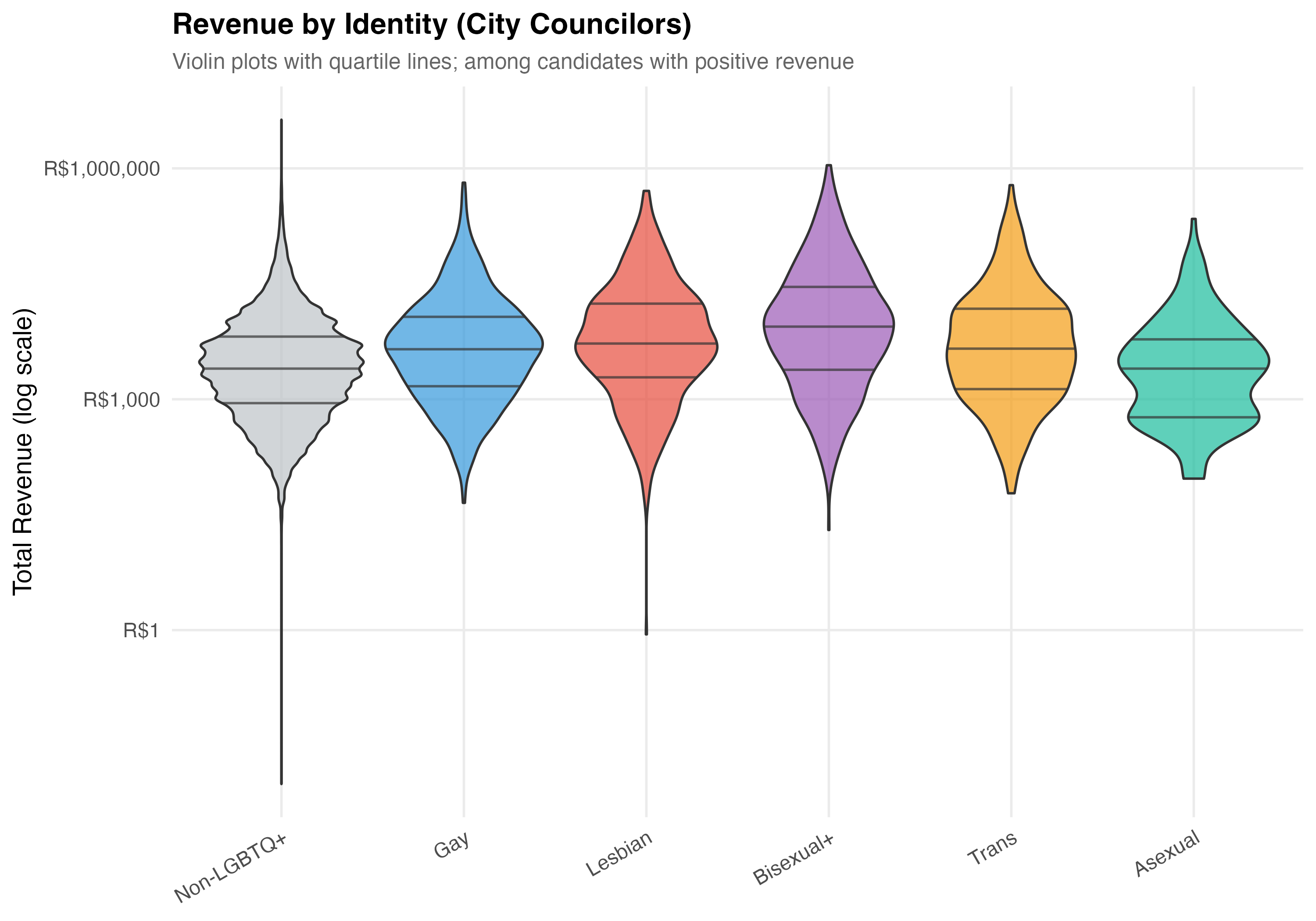
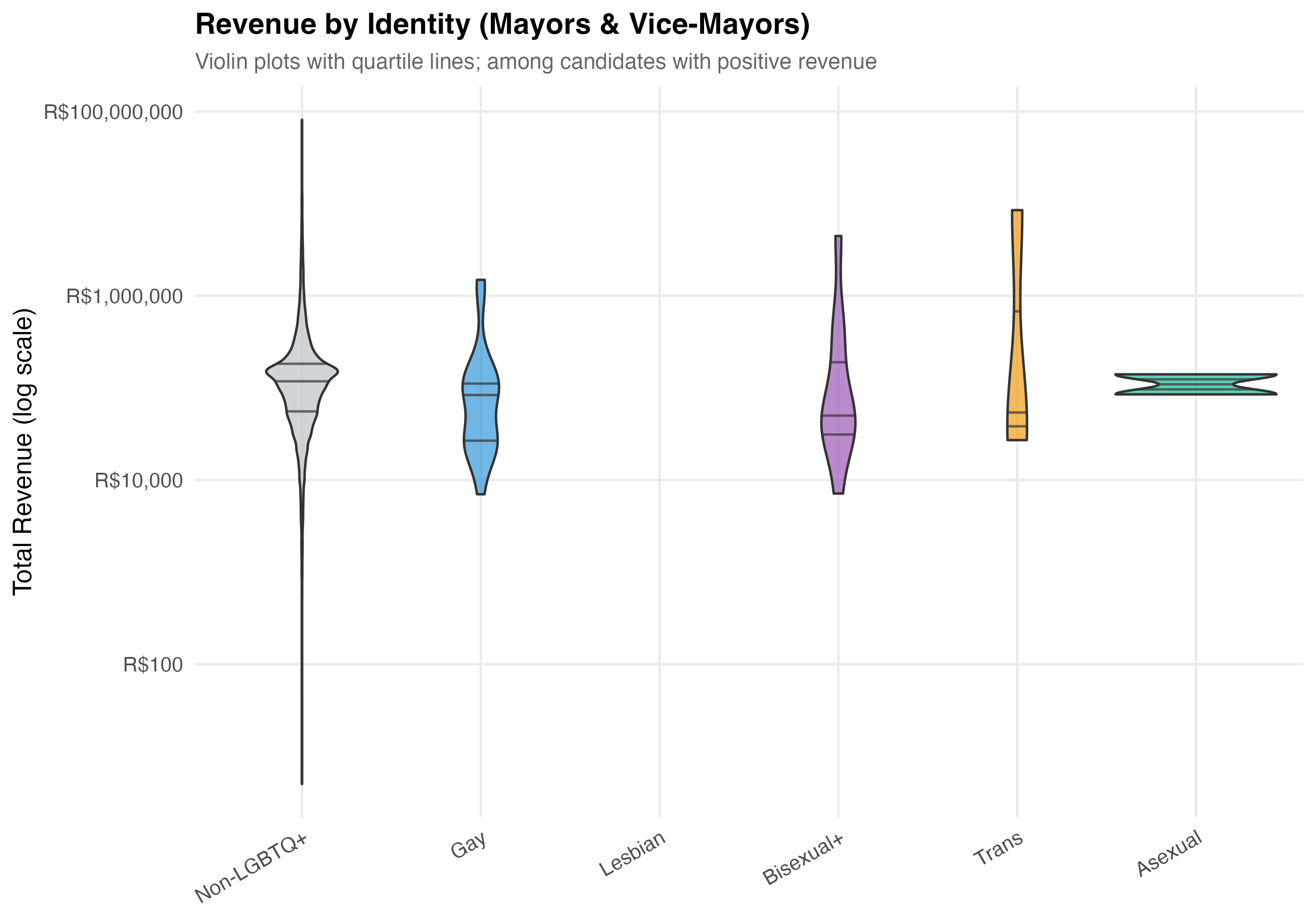
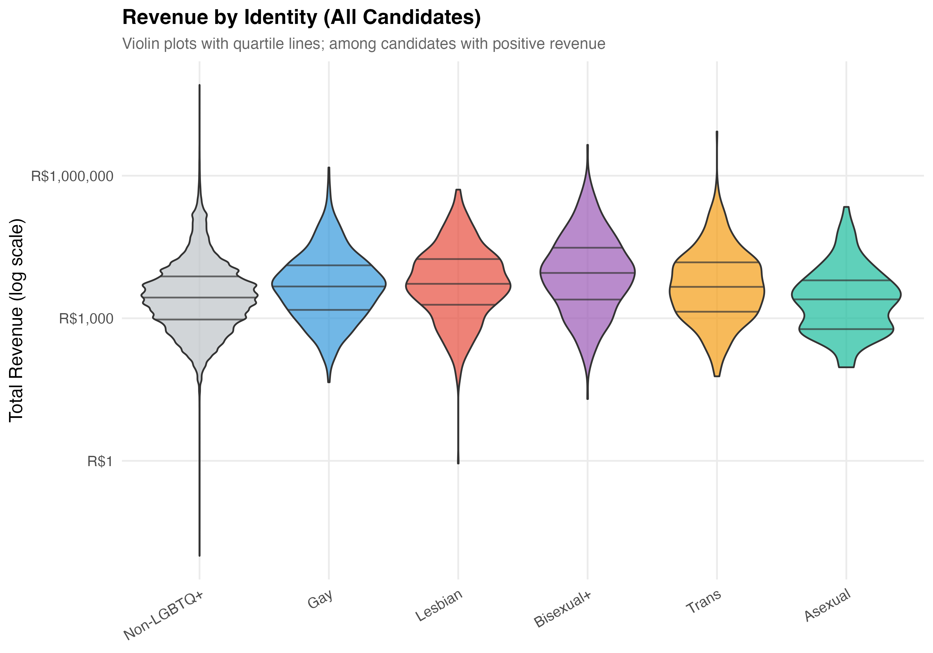
# --- Violin plot ---
cat("### Revenue Distribution by Category\n\n")
pos_rev <- data %>% filter(total_revenue > 0)
if (nrow(pos_rev) > 0) {
plot_data <- pos_rev %>%
mutate(
plot_category = if_else(lgbtq_candidate, as.character(lgbt_category), "Non-LGBTQ+"),
plot_category = factor(plot_category,
levels = c("Non-LGBTQ+", "Gay", "Lesbian", "Bisexual+",
"Trans", "Asexual"))
) %>%
filter(!is.na(plot_category))
if (simplified) {
# Small N: boxplot + jitter for LGBTQ+ categories
p_violin <- plot_data %>%
ggplot(aes(x = plot_category, y = total_revenue, fill = plot_category)) +
geom_boxplot(alpha = 0.7, outlier.shape = NA, width = 0.5) +
geom_jitter(data = . %>% filter(plot_category != "Non-LGBTQ+"),
alpha = 0.4, width = 0.15, size = 1) +
scale_y_log10(labels = label_dollar(prefix = "R$", big.mark = ",")) +
scale_fill_manual(values = pal_identity, guide = "none") +
labs(
x = NULL, y = "Total Revenue (log scale)",
title = paste0("Revenue by Identity (", tab_name, ")"),
subtitle = "Boxplot with individual LGBTQ+ observations"
) +
theme(axis.text.x = element_text(angle = 30, hjust = 1))
} else {
p_violin <- plot_data %>%
ggplot(aes(x = plot_category, y = total_revenue, fill = plot_category)) +
geom_violin(alpha = 0.7, draw_quantiles = c(0.25, 0.5, 0.75)) +
scale_y_log10(labels = label_dollar(prefix = "R$", big.mark = ",")) +
scale_fill_manual(values = pal_identity, guide = "none") +
labs(
x = NULL, y = "Total Revenue (log scale)",
title = paste0("Revenue by Identity (", tab_name, ")"),
subtitle = "Violin plots with quartile lines; among candidates with positive revenue"
) +
theme(axis.text.x = element_text(angle = 30, hjust = 1))
}
cat_plot(p_violin, paste0("05-violin-identity-", pos_suffix(tab_name)))
}
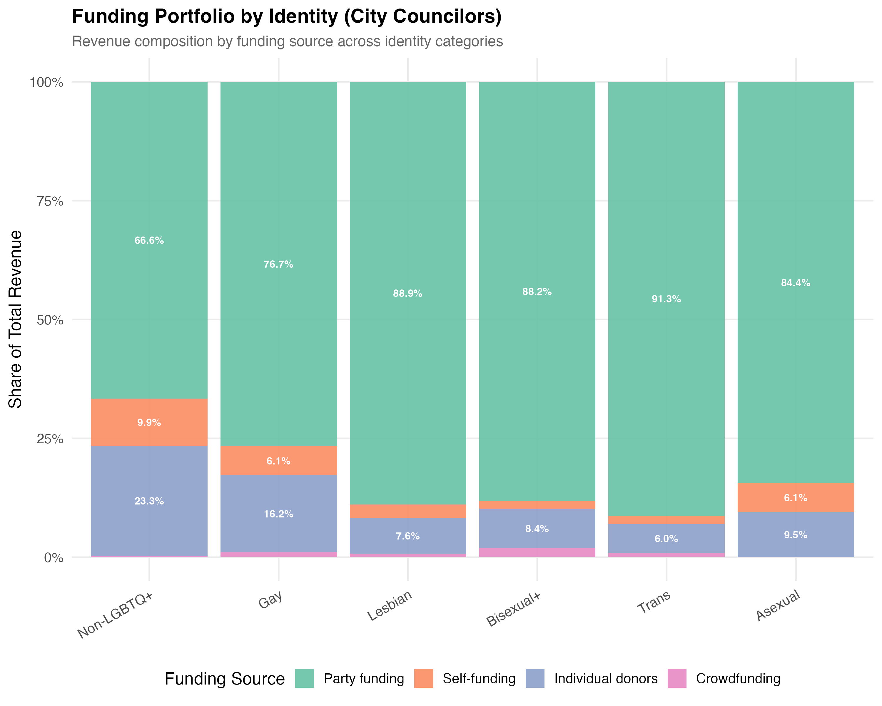
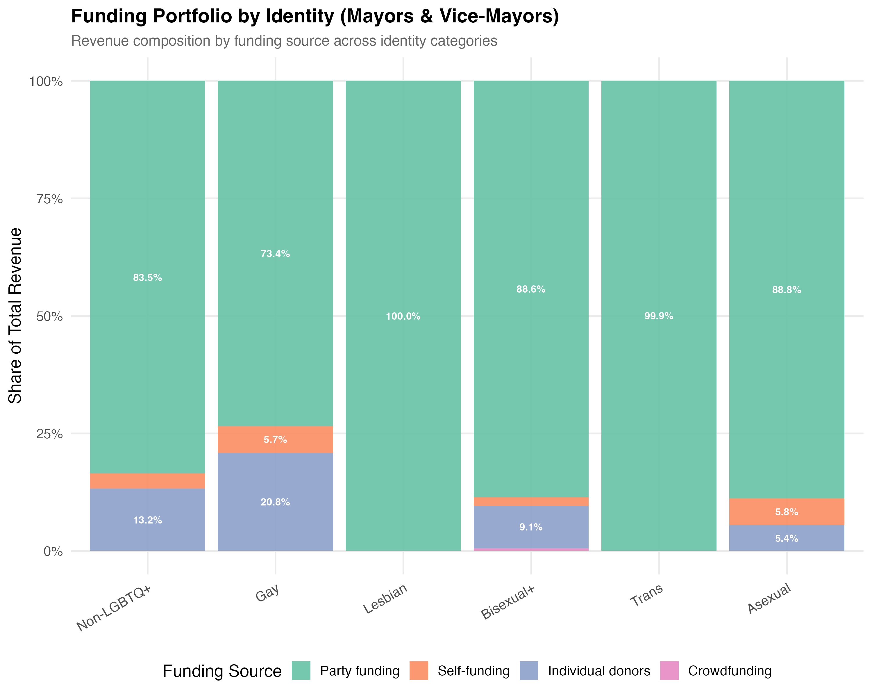
# --- Funding composition by identity ---
cat("### Funding Composition by Category\n\n")
comp_data <- data %>%
mutate(
plot_category = if_else(lgbtq_candidate, as.character(lgbt_category), "Non-LGBTQ+"),
plot_category = factor(plot_category,
levels = c("Non-LGBTQ+", "Gay", "Lesbian", "Bisexual+",
"Trans", "Asexual"))
) %>%
filter(!is.na(plot_category)) %>%
group_by(plot_category) %>%
summarise(
`Self-funding` = sum(self_funding_amt, na.rm = TRUE),
`Party funding` = sum(party_funding_amt, na.rm = TRUE),
`Individual donors` = sum(individual_funding_amt, na.rm = TRUE),
`Crowdfunding` = sum(crowdfunding_amt, na.rm = TRUE),
.groups = "drop"
) %>%
pivot_longer(-plot_category, names_to = "source", values_to = "total") %>%
group_by(plot_category) %>%
mutate(pct = total / sum(total)) %>%
ungroup() %>%
mutate(source = factor(source,
levels = c("Party funding", "Self-funding",
"Individual donors", "Crowdfunding")))
p_comp_id <- comp_data %>%
ggplot(aes(x = plot_category, y = pct, fill = source)) +
geom_col(alpha = 0.9) +
geom_text(aes(label = if_else(pct > 0.05, format_pct(pct), "")),
position = position_stack(vjust = 0.5), size = 3, color = "white",
fontface = "bold") +
scale_fill_brewer(palette = "Set2", name = "Funding Source") +
scale_y_continuous(labels = percent) +
labs(
x = NULL,
y = "Share of Total Revenue",
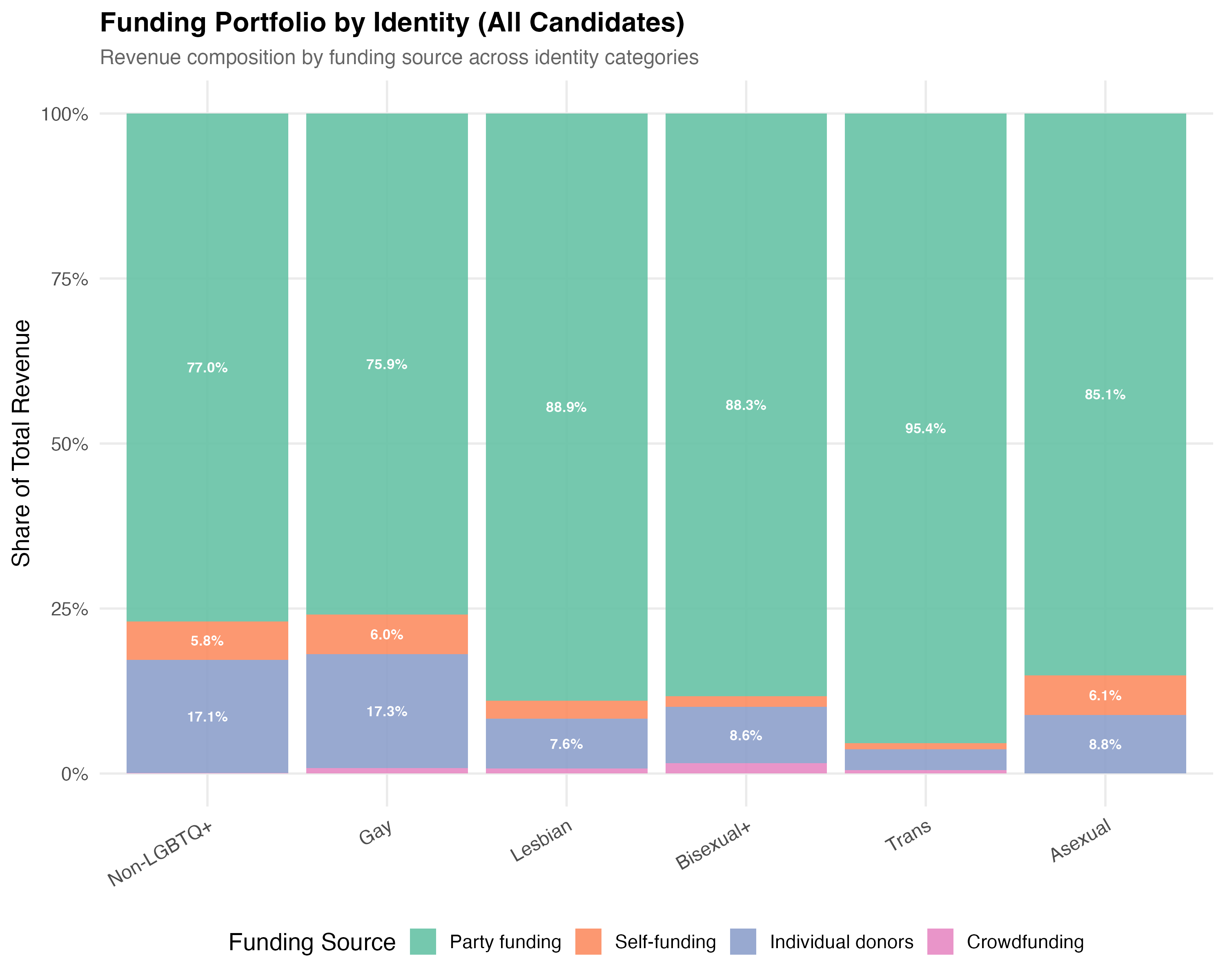
title = paste0("Funding Portfolio by Identity (", tab_name, ")"),
subtitle = "Revenue composition by funding source across identity categories"
) +
theme(axis.text.x = element_text(angle = 30, hjust = 1))
cat_plot(p_comp_id, paste0("05-composition-identity-", pos_suffix(tab_name)), height = 8)
# Position-specific within-group callout
id_stats <- data %>%
filter(lgbtq_candidate, lgbt_category != "Other LGBTQ+") %>%
group_by(lgbt_category) %>%
summarise(
mean_pct_party = mean(pct_party, na.rm = TRUE),
mean_pct_individual = mean(pct_individual, na.rm = TRUE),
.groups = "drop"
)
if (nrow(id_stats) > 0) {
top_p <- id_stats %>% slice_max(mean_pct_party, n = 1)
top_i <- id_stats %>% slice_max(mean_pct_individual, n = 1)
cat("::: {.callout-note}\n")
cat("## Within-Group Differences\n")
cat(sprintf("In this tab (%s), %s candidates have the highest average party funding share (%s), ",
tab_name, top_p$lgbt_category, format_pct100(top_p$mean_pct_party)))
cat(sprintf("while %s candidates have the highest average individual donor share (%s).\n",
top_i$lgbt_category, format_pct100(top_i$mean_pct_individual)))
cat(":::\n\n")
}
}
render_position_tabset(render_identity_revenue, df)
```
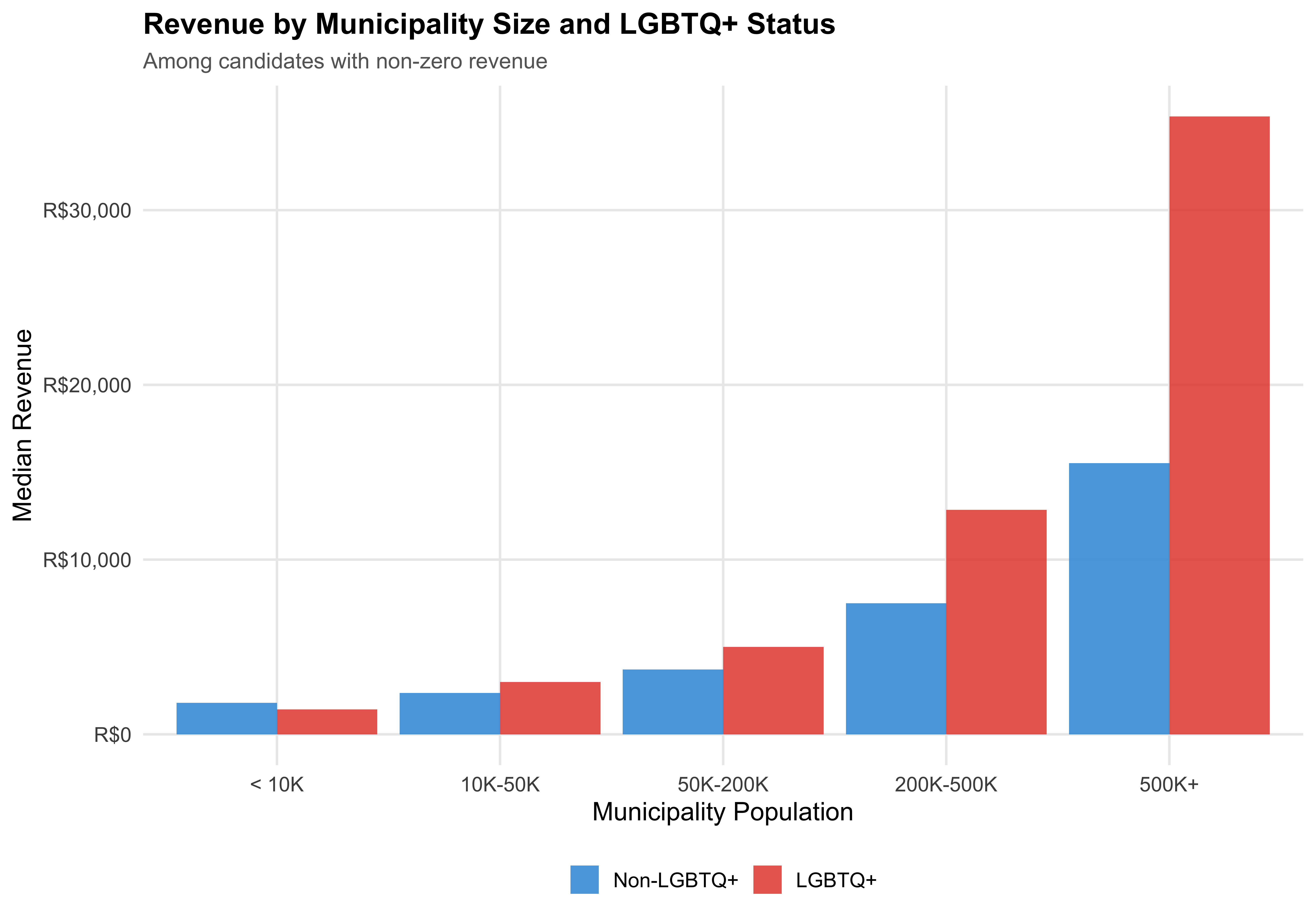
# Revenue by Municipality Size
LGBTQ+ candidates tend to run in larger, more urbanized municipalities (see [Chapter 4](04_geography.qmd)). Since larger cities have more expensive campaigns, a naive revenue comparison may overstate LGBTQ+ fundraising capacity. This section compares revenue *within* population brackets to reveal whether the aggregate pattern holds when municipality size is accounted for.
```{r tbl-revenue-pop}
#| label: tbl-revenue-pop
#| tbl-cap: "Median Revenue by Municipality Population and LGBTQ+ Status"
rev_by_pop <- df %>%
  filter(!is.na(pop_bracket), total_revenue > 0) %>%
  group_by(pop_bracket, lgbtq_label) %>%
  summarise(
    N = n(),
    median_rev = median(total_revenue, na.rm = TRUE),
    mean_rev   = mean(total_revenue, na.rm = TRUE),
    .groups = "drop"
  )

rev_by_pop_wide <- rev_by_pop %>%
  select(pop_bracket, lgbtq_label, N, median_rev) %>%
  pivot_wider(names_from = lgbtq_label,
              values_from = c(N, median_rev),
              names_sep = "_") %>%
  mutate(
    ratio = round(`median_rev_LGBTQ+` / `median_rev_Non-LGBTQ+`, 2)
  )

rev_by_pop_wide %>%
  transmute(
    `Pop. Bracket` = pop_bracket,
    `N LGBTQ+` = format_n(`N_LGBTQ+`),
    `Median LGBTQ+` = format_brl(`median_rev_LGBTQ+`),
    `N Non-LGBTQ+` = format_n(`N_Non-LGBTQ+`),
    `Median Non-LGBTQ+` = format_brl(`median_rev_Non-LGBTQ+`),
    `Ratio` = ratio
  ) %>%
  kable(align = c("l", rep("r", 5)))
```
```{r fig-revenue-pop}
#| label: fig-revenue-pop
#| fig-cap: "Median Revenue by Municipality Size and LGBTQ+ Status"
ggplot(rev_by_pop, aes(x = pop_bracket, y = median_rev, fill = lgbtq_label)) +
  geom_col(position = "dodge", alpha = 0.85) +
  scale_y_continuous(labels = scales::label_dollar(prefix = "R$", big.mark = ",")) +
  scale_fill_manual(values = pal_lgbtq) +
  labs(
    x = "Municipality Population",
    y = "Median Revenue",
    fill = NULL,
    title = "Revenue by Municipality Size and LGBTQ+ Status",
    subtitle = "Among candidates with non-zero revenue"
  )

save_figure(last_plot(), "05_revenue_by_pop_bracket")
```
::: {.callout-note}
## Selection into Larger Markets
LGBTQ+ candidates disproportionately run in larger municipalities where campaigns are more expensive. The aggregate revenue comparison may therefore obscure the within-market fundraising gap. Compare the overall median ratio with the bracket-specific ratios above.
:::
::: {.callout-note}
## Pooled Across Positions
This section pools across position types because the analysis controls for municipality size directly. The comparison examines whether LGBTQ+ candidates raise more or less than non-LGBTQ+ counterparts *within the same population bracket*, making position disaggregation less critical. Mayoral campaigns operate at a fundamentally different revenue scale; the position-specific tabs in earlier sections capture this difference.
:::
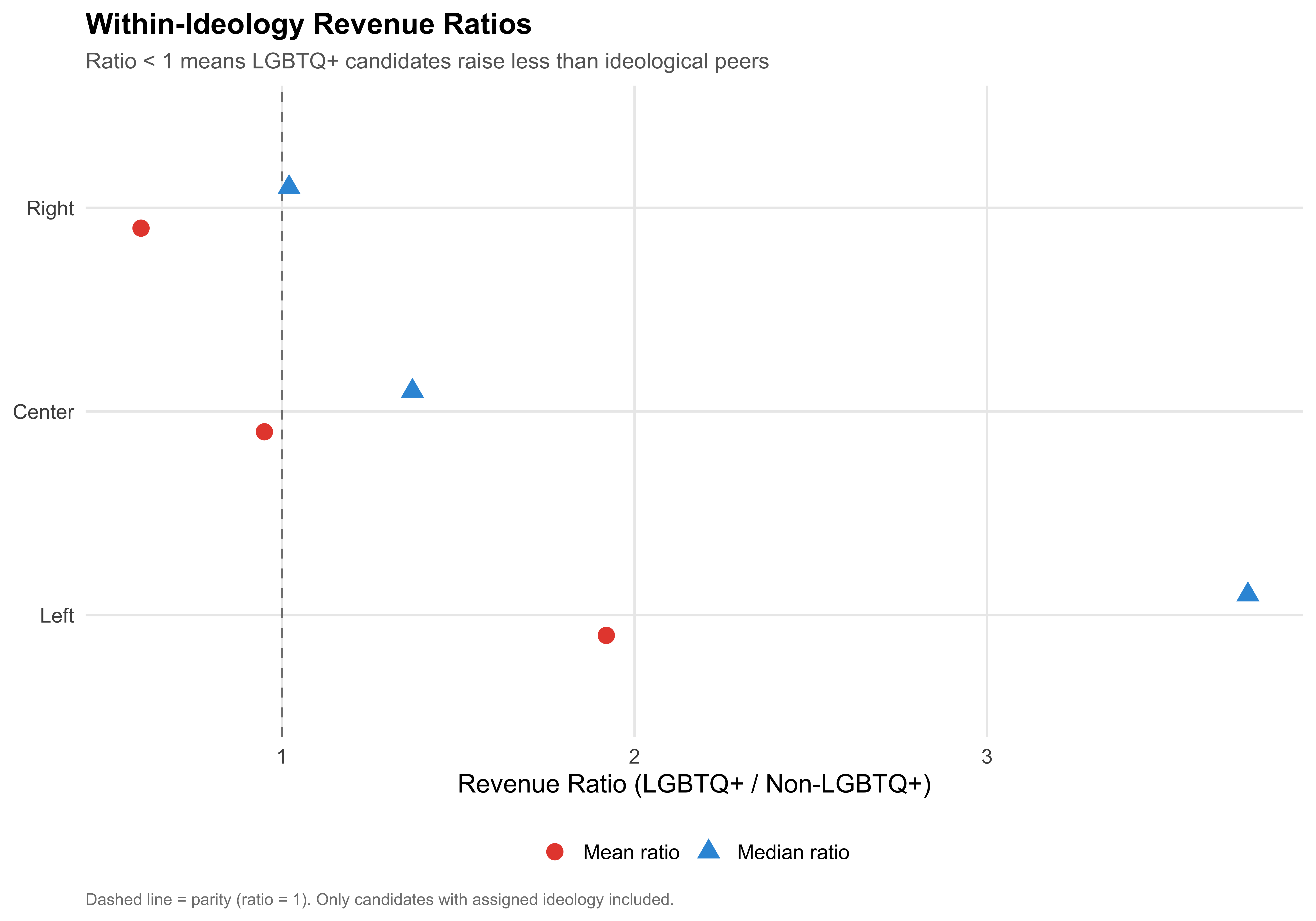
# Within-Ideology Comparison
The within-ideology revenue ratio compares LGBTQ+ and non-LGBTQ+ candidates *within the same ideological bloc* (Left, Center, Right). The ratio is computed as LGBTQ+ mean (or median) revenue divided by non-LGBTQ+ mean (or median) revenue for each bloc. A ratio below 1 means LGBTQ+ candidates raise less than their ideological peers; a ratio above 1 means they raise more.
```{r tbl-within-ideology}
#| label: tbl-within-ideology
#| tbl-cap: "Revenue Comparison Within Ideological Blocs (LGBTQ+ vs Non-LGBTQ+)"
within_ideo <- df %>%
  filter(!is.na(ideology_category)) %>%
  mutate(group = if_else(lgbtq_candidate, "LGBTQ+", "Non-LGBTQ+")) %>%
  group_by(ideology_category, group) %>%
  summarise(
    N          = n(),
    mean_rev   = mean(total_revenue, na.rm = TRUE),
    median_rev = median(total_revenue, na.rm = TRUE),
    .groups    = "drop"
  )

within_ideo_wide <- within_ideo %>%
  select(ideology_category, group, N, mean_rev, median_rev) %>%
  pivot_wider(
    names_from  = group,
    values_from = c(N, mean_rev, median_rev),
    names_glue  = "{group}_{.value}"
  ) %>%
  mutate(
    mean_ratio   = if_else(`Non-LGBTQ+_mean_rev` > 0,
                           round(`LGBTQ+_mean_rev` / `Non-LGBTQ+_mean_rev`, 2), NA_real_),
    median_ratio = if_else(`Non-LGBTQ+_median_rev` > 0,
                           round(`LGBTQ+_median_rev` / `Non-LGBTQ+_median_rev`, 2), NA_real_)
  ) %>%
  mutate(ideology_category = factor(ideology_category, levels = ideology_levels)) %>%
  arrange(ideology_category)

within_ideo_wide %>%
  transmute(
    Ideology                  = ideology_category,
    `N LGBTQ+`               = format_n(`LGBTQ+_N`),
    `N Non-LGBTQ+`           = format_n(`Non-LGBTQ+_N`),
    `Mean Rev. LGBTQ+`       = format_brl(`LGBTQ+_mean_rev`),
    `Mean Rev. Non-LGBTQ+`   = format_brl(`Non-LGBTQ+_mean_rev`),
    `Mean Ratio (L/NL)`      = if_else(is.na(mean_ratio), "---", as.character(mean_ratio)),
    `Median Rev. LGBTQ+`     = format_brl(`LGBTQ+_median_rev`),
    `Median Rev. Non-LGBTQ+` = format_brl(`Non-LGBTQ+_median_rev`),
    `Median Ratio (L/NL)`    = if_else(is.na(median_ratio), "---", as.character(median_ratio))
  ) %>%
  kable(align = c("l", "r", "r", "r", "r", "r", "r", "r", "r"))
```
```{r fig-within-ideology}
#| label: fig-within-ideology
#| fig-cap: "LGBTQ+/Non-LGBTQ+ Revenue Ratio Within Ideological Blocs"
plot_data <- within_ideo_wide %>%
  filter(!is.na(mean_ratio) | !is.na(median_ratio)) %>%
  select(ideology_category, `Mean ratio` = mean_ratio, `Median ratio` = median_ratio) %>%
  pivot_longer(-ideology_category, names_to = "metric", values_to = "ratio") %>%
  filter(!is.na(ratio))

ggplot(plot_data, aes(x = ideology_category, y = ratio,
           color = metric, shape = metric)) +
  geom_hline(yintercept = 1, linetype = "dashed", color = "gray50") +
  geom_point(size = 4, position = position_dodge(width = 0.4)) +
  coord_flip() +
  scale_color_manual(values = c("Mean ratio" = "#E74C3C", "Median ratio" = "#3498DB"),
                     name = NULL) +
  scale_shape_manual(values = c("Mean ratio" = 16, "Median ratio" = 17),
                     name = NULL) +
  labs(
    x       = NULL,
    y       = "Revenue Ratio (LGBTQ+ / Non-LGBTQ+)",
    title   = "Within-Ideology Revenue Ratios",
    subtitle = "Ratio < 1 means LGBTQ+ candidates raise less than ideological peers",
    caption  = "Dashed line = parity (ratio = 1). Only candidates with assigned ideology included."
  )

save_figure(last_plot(), "05_within_ideology_ratio")
```
```{r within-ideology-inline}
n_ideo_below1_mean   <- sum(within_ideo_wide$mean_ratio < 1, na.rm = TRUE)
n_ideo_above1_mean   <- sum(within_ideo_wide$mean_ratio > 1, na.rm = TRUE)
n_ideo_below1_median <- sum(within_ideo_wide$median_ratio < 1, na.rm = TRUE)
n_ideo_total         <- nrow(within_ideo_wide)
```
::: {.callout-note}
## Within-Ideology Revenue Ratios
Of the `r n_ideo_total` ideological blocs, `r n_ideo_below1_mean` show a mean revenue ratio below 1 (LGBTQ+ candidates raising less than ideological peers) and `r n_ideo_above1_mean` show a mean ratio above 1. At the median, `r n_ideo_below1_median` of `r n_ideo_total` blocs have ratios below 1.
:::
::: {.callout-note}
## Pooled Across Positions
The within-ideology revenue comparison pools across position types because it already conditions on a key confounder (ideology). Position-specific results for the LGBTQ+ vs. non-LGBTQ+ revenue comparison are available in the tabbed section above.
:::
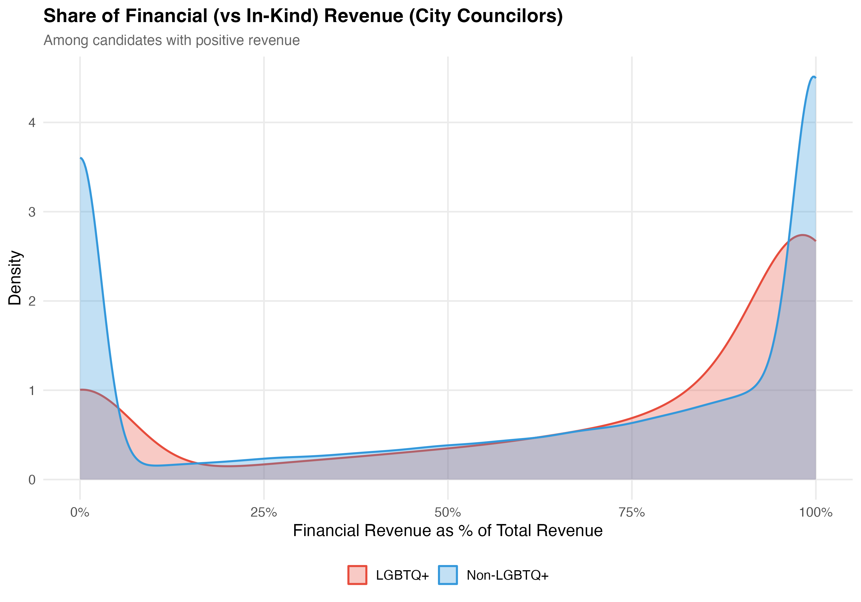
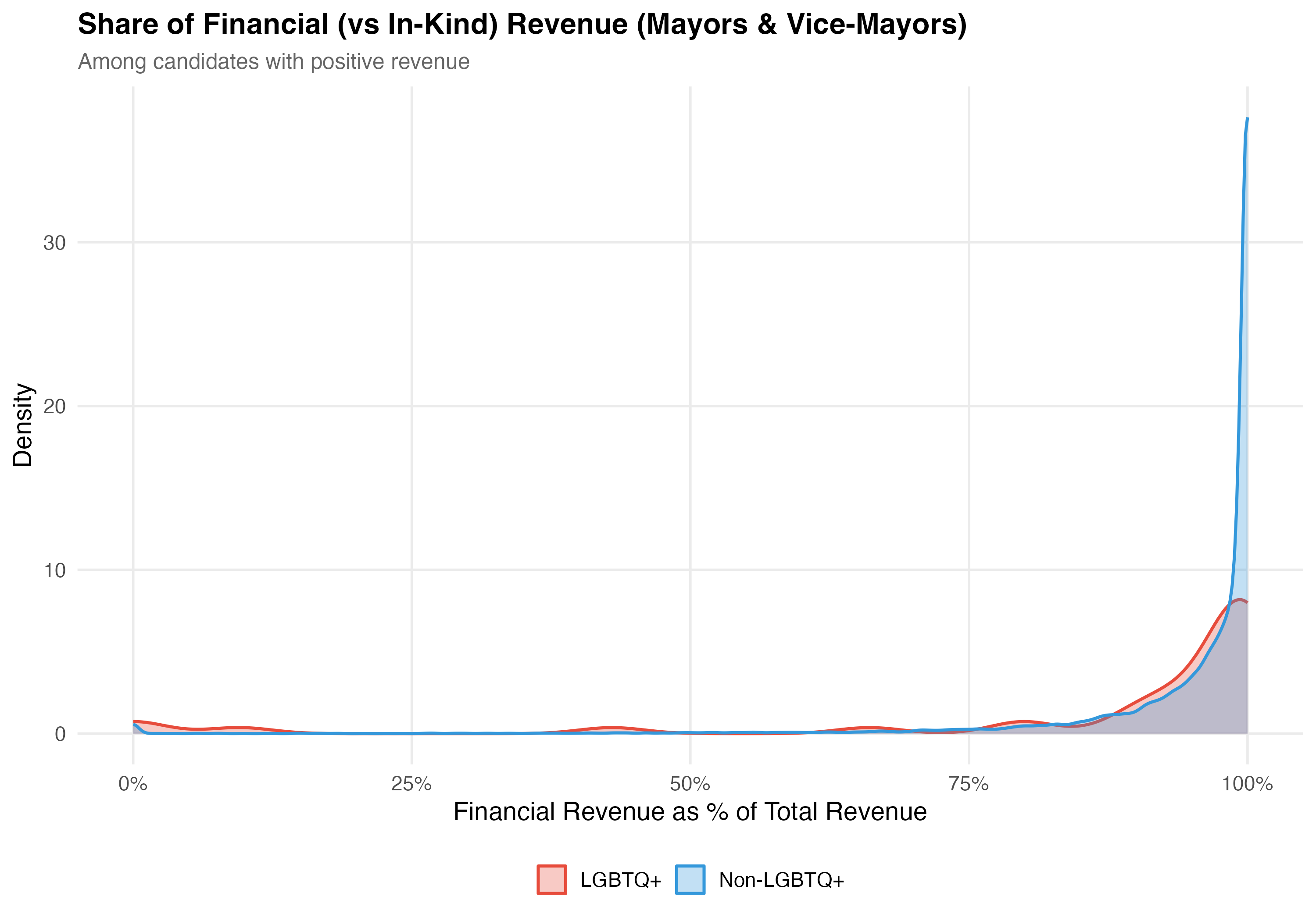
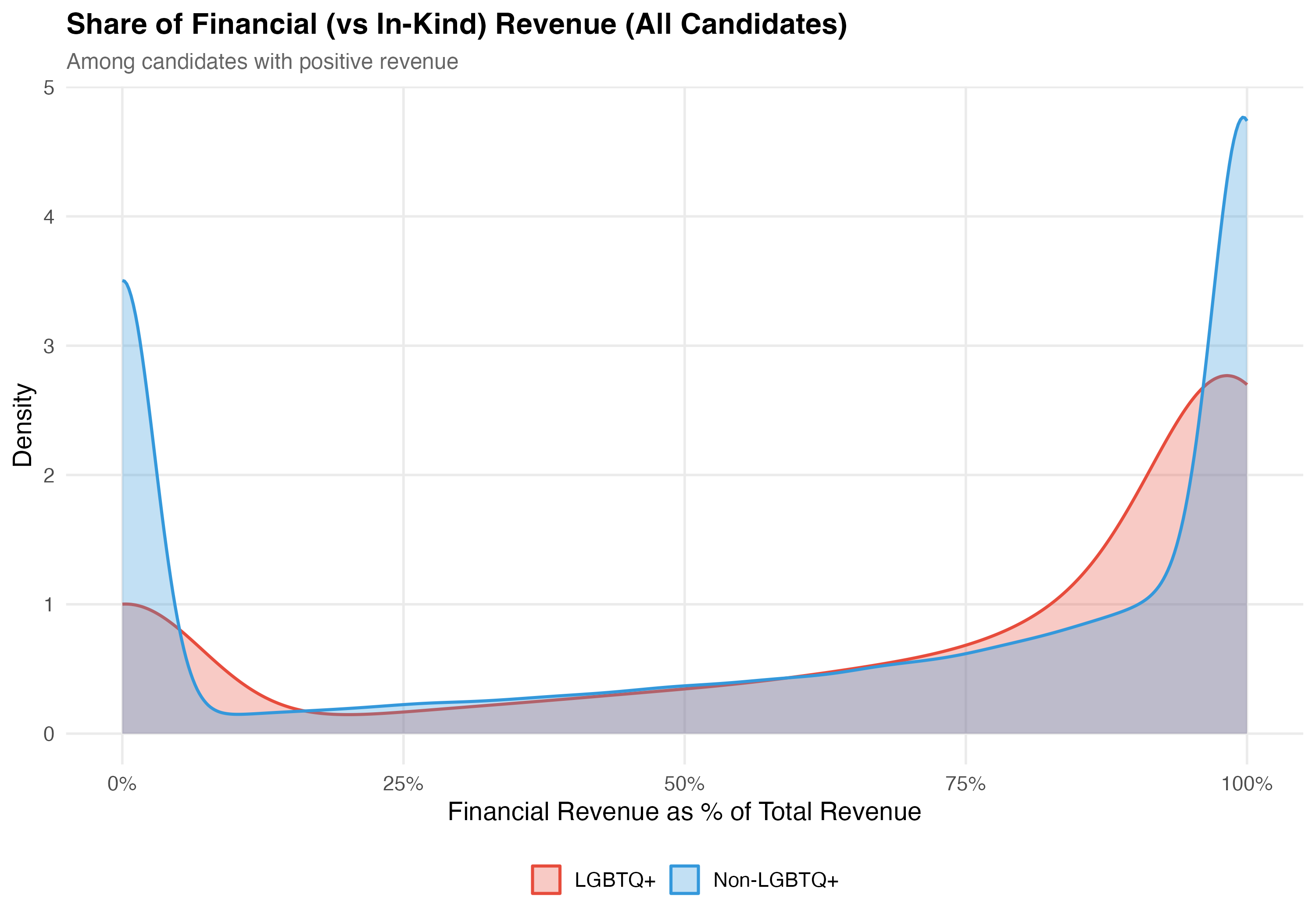
# Financial vs In-Kind Contributions
The TSE classifies each transaction's `DS_NATUREZA_RECEITA` as either "FINANCEIRO" (financial) or a non-financial category. **Financial contributions** are direct monetary transfers: cash, PIX, bank deposits, and electronic transfers. **In-kind contributions** (*recursos estimaveis*) are non-monetary --- goods, services, or volunteer labor that the campaign assigns a monetary value to for accounting purposes. Examples include donated office space, printing services, vehicles for campaign use, or professional labor contributed without charge. The variables `pct_financial` and `pct_inkind` express each type's share of a candidate's total revenue on a 0--100 scale.
```{r financial-inkind-tabset}
#| results: asis
render_financial_inkind <- function(data, tab_name) {
# --- Financial vs In-Kind comparison table ---
cat("### Financial vs In-Kind Revenue\n\n")
data %>%
mutate(group = if_else(lgbtq_candidate, "LGBTQ+", "Non-LGBTQ+")) %>%
group_by(group) %>%
summarise(
N = format_n(n()),
`Total Financial` = format_brl(sum(financial_amt, na.rm = TRUE)),
`Total In-Kind` = format_brl(sum(inkind_amt, na.rm = TRUE)),
`Mean % Financial` = format_pct100(mean(pct_financial, na.rm = TRUE)),
`Mean % In-Kind` = format_pct100(mean(pct_inkind, na.rm = TRUE)),
`Median % Financial` = format_pct100(median(pct_financial, na.rm = TRUE)),
`Median % In-Kind` = format_pct100(median(pct_inkind, na.rm = TRUE)),
.groups = "drop"
) %>%
rename(Group = group) %>%
cat_kable(align = c("l", "r", "r", "r", "r", "r", "r", "r"))
# --- Density plot of financial share ---
cat("### Financial Share Distribution\n\n")
pos_rev <- data %>% filter(total_revenue > 0)
if (nrow(pos_rev) > 0) {
p_density <- pos_rev %>%
mutate(group = if_else(lgbtq_candidate, "LGBTQ+", "Non-LGBTQ+")) %>%
ggplot(aes(x = pct_financial / 100, fill = group, color = group)) +
geom_density(alpha = 0.3, linewidth = 0.8) +
scale_fill_manual(values = pal_lgbtq, name = NULL) +
scale_color_manual(values = pal_lgbtq, name = NULL) +
scale_x_continuous(labels = percent, limits = c(0, 1)) +
labs(
x = "Financial Revenue as % of Total Revenue",
y = "Density",
title = paste0("Share of Financial (vs In-Kind) Revenue (", tab_name, ")"),
subtitle = "Among candidates with positive revenue"
)
cat_plot(p_density, paste0("05-financial-inkind-density-", pos_suffix(tab_name)))
}
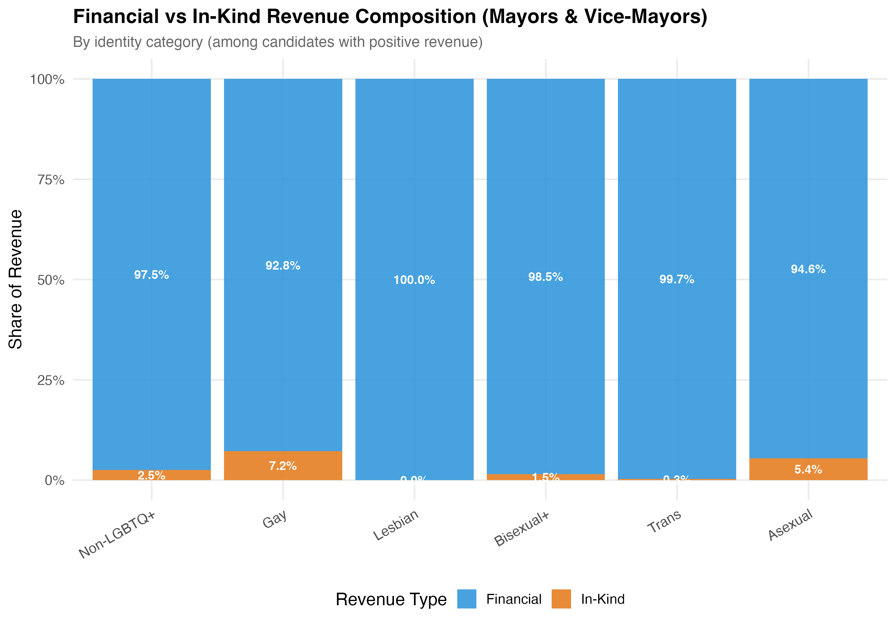
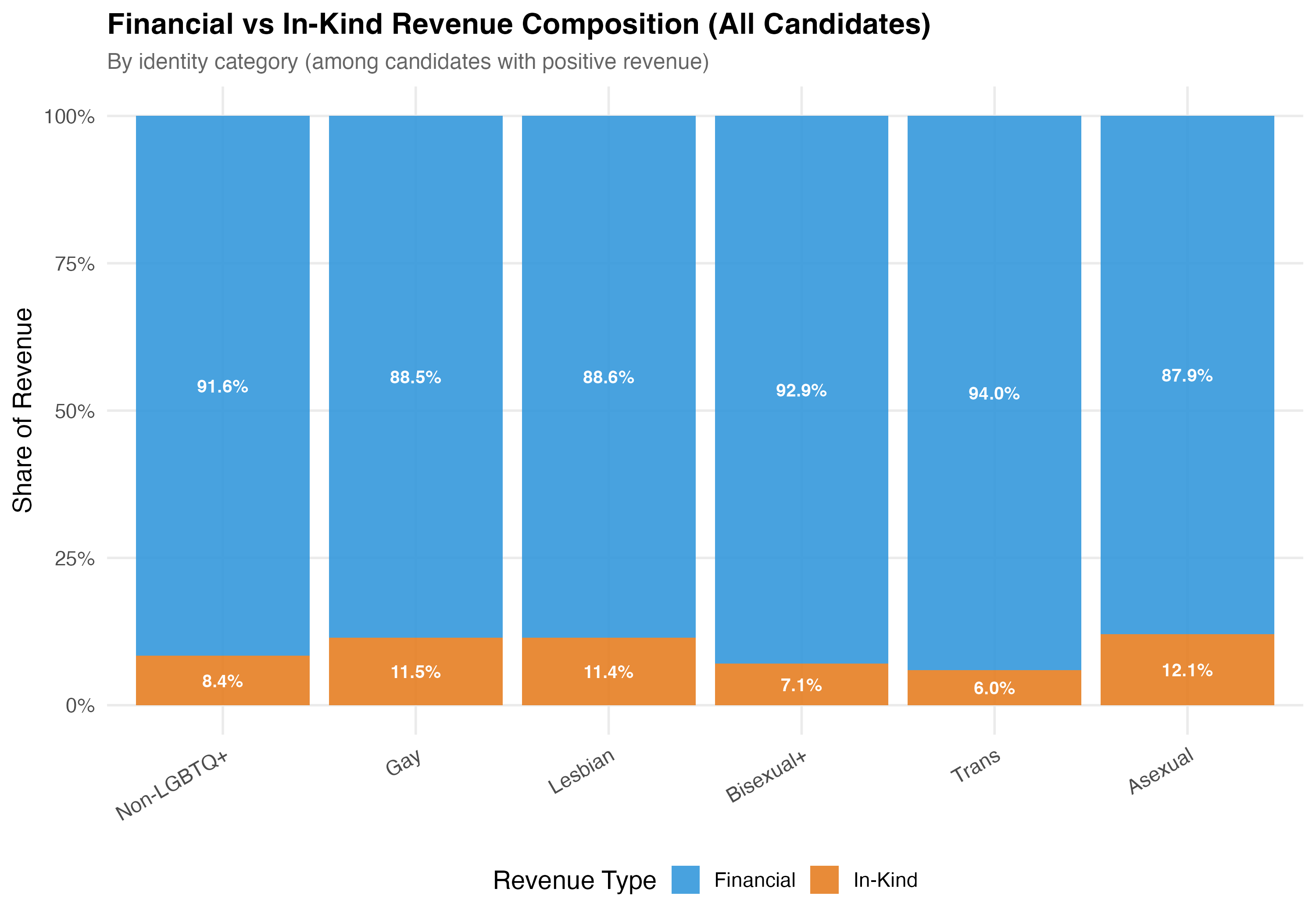
# --- Stacked bar by identity category ---
cat("### Financial vs In-Kind by Identity\n\n")
p_identity <- data %>%
filter(total_revenue > 0) %>%
mutate(
plot_category = if_else(lgbtq_candidate, as.character(lgbt_category), "Non-LGBTQ+"),
plot_category = factor(plot_category,
levels = c("Non-LGBTQ+", "Gay", "Lesbian", "Bisexual+",
"Trans", "Asexual"))
) %>%
filter(!is.na(plot_category)) %>%
group_by(plot_category) %>%
summarise(
Financial = sum(financial_amt, na.rm = TRUE),
`In-Kind` = sum(inkind_amt, na.rm = TRUE),
.groups = "drop"
) %>%
pivot_longer(-plot_category, names_to = "type", values_to = "total") %>%
group_by(plot_category) %>%
mutate(pct = total / sum(total)) %>%
ungroup() %>%
ggplot(aes(x = plot_category, y = pct, fill = type)) +
geom_col(alpha = 0.9) +
geom_text(aes(label = format_pct(pct)),
position = position_stack(vjust = 0.5), size = 3.5, color = "white",
fontface = "bold") +
scale_fill_manual(values = c("Financial" = "#3498DB", "In-Kind" = "#E67E22"),
name = "Revenue Type") +
scale_y_continuous(labels = percent) +
labs(
x = NULL,
y = "Share of Revenue",
title = paste0("Financial vs In-Kind Revenue Composition (", tab_name, ")"),
subtitle = "By identity category (among candidates with positive revenue)"
) +
theme(axis.text.x = element_text(angle = 30, hjust = 1))
cat_plot(p_identity, paste0("05-financial-inkind-identity-", pos_suffix(tab_name)))
cat("::: {.callout-note}\n")
cat("## Financial vs. In-Kind\n")
cat("Financial contributions are direct monetary transfers (cash, PIX, bank transfers). ")
cat("In-kind contributions are non-monetary goods and services assigned a monetary value ")
cat("for accounting purposes. The table and density plot above compare these two categories ")
cat("across LGBTQ+ and non-LGBTQ+ candidates.\n")
cat(":::\n\n")
}
render_position_tabset(render_financial_inkind, df)
```
::: {.callout-note}
## Pooled Across Positions
The in-kind contribution type analysis below pools across city councilors and mayors/vice-mayors. This section examines transaction-level data (individual contribution records) rather than candidate-level aggregates, and the types of in-kind support received do not vary systematically by position type.
:::
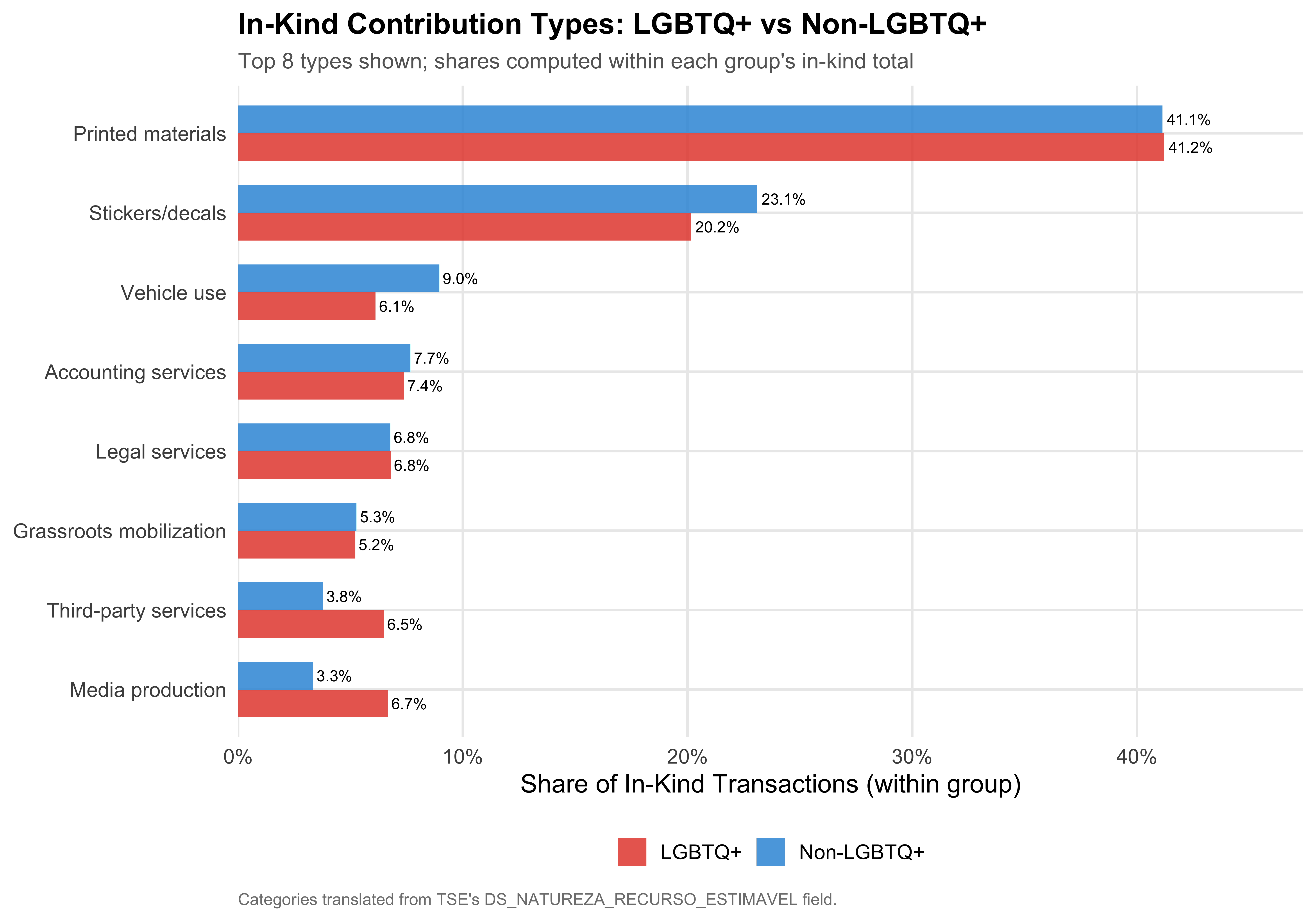
## Types of In-Kind Contributions
The TSE records the specific type of each in-kind contribution in the field `DS_NATUREZA_RECURSO_ESTIMAVEL`. This variable is only populated for non-financial transactions and describes the nature of the donated good or service (e.g., advertising materials, vehicles, professional services). This section examines which types of in-kind support are most common and whether the composition differs between LGBTQ+ and non-LGBTQ+ candidates.
```{r inkind-data}
# Filter transaction-level data to in-kind contributions
inkind_trans <- receitas %>%
  filter(DS_NATUREZA_RECEITA != "FINANCEIRO") %>%
  filter(!is.na(DS_NATUREZA_RECURSO_ESTIMAVEL),
         DS_NATUREZA_RECURSO_ESTIMAVEL != "#NULO#",
         DS_NATUREZA_RECURSO_ESTIMAVEL != "#NULO")

# Join with df to get LGBTQ+ flag (candidate_id in df == SQ_CANDIDATO in transactions)
inkind_trans <- inkind_trans %>%
  inner_join(
    df %>% select(candidate_id, lgbtq_candidate),
    by = c("SQ_CANDIDATO" = "candidate_id")
  ) %>%
  mutate(group = if_else(lgbtq_candidate, "LGBTQ+", "Non-LGBTQ+"))

# Translate and group Portuguese categories into English labels
# Top categories get their own label; rare categories are grouped
inkind_trans <- inkind_trans %>%
  mutate(
    inkind_en = case_when(
      str_detect(DS_NATUREZA_RECURSO_ESTIMAVEL, "materiais impressos")   ~ "Printed materials",
      str_detect(DS_NATUREZA_RECURSO_ESTIMAVEL, "adesivos")              ~ "Stickers/decals",
      str_detect(DS_NATUREZA_RECURSO_ESTIMAVEL, "veículos")              ~ "Vehicle use",
      str_detect(DS_NATUREZA_RECURSO_ESTIMAVEL, "contábeis")             ~ "Accounting services",
      str_detect(DS_NATUREZA_RECURSO_ESTIMAVEL, "advocatícios")          ~ "Legal services",
      str_detect(DS_NATUREZA_RECURSO_ESTIMAVEL, "militância")            ~ "Grassroots mobilization",
      str_detect(DS_NATUREZA_RECURSO_ESTIMAVEL, "rádio|televisão|vídeo") ~ "Media production",
      str_detect(DS_NATUREZA_RECURSO_ESTIMAVEL, "terceiros")             ~ "Third-party services",
      str_detect(DS_NATUREZA_RECURSO_ESTIMAVEL, "pessoal")               ~ "Personnel costs",
      str_detect(DS_NATUREZA_RECURSO_ESTIMAVEL, "jingles|vinhetas")      ~ "Jingles/slogans",
      str_detect(DS_NATUREZA_RECURSO_ESTIMAVEL, "bens imóveis")          ~ "Property rental",
      TRUE                                                               ~ "Other"
    )
  )
```
```{r tbl-inkind-types}
#| label: tbl-inkind-types
#| tbl-cap: "Top In-Kind Contribution Types (All Candidates)"
inkind_freq <- inkind_trans %>%
  group_by(inkind_en) %>%
  summarise(
    n = n(),
    total_amt = sum(VR_RECEITA, na.rm = TRUE),
    mean_amt  = mean(VR_RECEITA, na.rm = TRUE),
    .groups = "drop"
  ) %>%
  arrange(desc(n)) %>%
  mutate(
    pct = n / sum(n),
    cum_pct = cumsum(pct),
    pct_amt = total_amt / sum(total_amt)
  )

n_inkind_types_raw <- inkind_trans %>%
  pull(DS_NATUREZA_RECURSO_ESTIMAVEL) %>%
  n_distinct()

inkind_freq %>%
  mutate(
    `N Transactions` = format_n(n),
    `% Trans.` = format_pct(pct),
    `Total (R$)` = format_brl(total_amt),
    `% Value` = format_pct(pct_amt),
    `Mean (R$)` = format_brl(mean_amt)
  ) %>%
  select(
    `In-Kind Type` = inkind_en,
    `N Transactions`,
    `% Trans.`,
    `Total (R$)`,
    `% Value`,
    `Mean (R$)`
  ) %>%
  kable(align = c("l", "r", "r", "r", "r", "r"))
```
```{r inkind-inline}
# Top in-kind type
top_inkind_type <- inkind_freq$inkind_en[1]
top_inkind_pct  <- inkind_freq$pct[1]
second_inkind_type <- inkind_freq$inkind_en[2]
second_inkind_pct  <- inkind_freq$pct[2]
top6_cum <- inkind_freq$cum_pct[min(6, nrow(inkind_freq))]
```
The TSE records `r n_inkind_types_raw` distinct in-kind categories; we group these into `r nrow(inkind_freq)` English-translated types for readability. The two largest --- **`r top_inkind_type`** (`r format_pct(top_inkind_pct)`) and **`r second_inkind_type`** (`r format_pct(second_inkind_pct)`) --- together account for nearly `r format_pct(inkind_freq$cum_pct[2])` of all in-kind transactions. The top six types cover `r format_pct(top6_cum)`.
### In-Kind Value by LGBTQ+ Status and Identity
```{r tbl-inkind-by-identity}
#| label: tbl-inkind-by-identity
#| tbl-cap: "In-Kind Contribution Value by LGBTQ+ Status and Identity Category"
# Join identity to in-kind transactions
inkind_identity <- inkind_trans %>%
  inner_join(
    df %>% select(candidate_id, lgbt_category),
    by = c("SQ_CANDIDATO" = "candidate_id")
  )

inkind_by_group <- inkind_identity %>%
  mutate(
    display_group = if_else(lgbtq_candidate, as.character(lgbt_category), "Non-LGBTQ+")
  ) %>%
  group_by(display_group) %>%
  summarise(
    `N Transactions` = n(),
    `Total (R$)` = format_brl(sum(VR_RECEITA, na.rm = TRUE)),
    `Mean (R$)` = format_brl(mean(VR_RECEITA, na.rm = TRUE)),
    `Median (R$)` = format_brl(median(VR_RECEITA, na.rm = TRUE)),
    .groups = "drop"
  )

inkind_by_group %>%
  rename(Group = display_group) %>%
  kable(align = c("l", "r", "r", "r", "r"),
        format.args = list(big.mark = ","))
```
```{r fig-inkind-types}
#| label: fig-inkind-types
#| fig-cap: "Top In-Kind Contribution Types: LGBTQ+ vs Non-LGBTQ+"
#| fig-height: 7
# Compute shares by group for the top types (excluding "Other")
top_labels <- inkind_freq %>%
  filter(inkind_en != "Other") %>%
  head(8) %>%
  pull(inkind_en)

inkind_by_group <- inkind_trans %>%
  filter(inkind_en %in% top_labels) %>%
  count(group, inkind_en) %>%
  group_by(group) %>%
  mutate(pct = n / sum(n)) %>%
  ungroup() %>%
  mutate(inkind_en = factor(inkind_en, levels = rev(top_labels)))

ggplot(inkind_by_group, aes(x = pct, y = inkind_en, fill = group)) +
  geom_col(position = "dodge", alpha = 0.85, width = 0.7) +
  geom_text(aes(label = format_pct(pct)),
            position = position_dodge(width = 0.7), hjust = -0.1,
            size = 3) +
  scale_fill_manual(values = pal_lgbtq, name = NULL) +
  scale_x_continuous(labels = percent, expand = expansion(mult = c(0, 0.15))) +
  labs(
    x        = "Share of In-Kind Transactions (within group)",
    y        = NULL,
    title    = "In-Kind Contribution Types: LGBTQ+ vs Non-LGBTQ+",
    subtitle = "Top 8 types shown; shares computed within each group's in-kind total",
    caption  = "Categories translated from TSE's DS_NATUREZA_RECURSO_ESTIMAVEL field."
  )

save_figure(last_plot(), "05_inkind_types_comparison", height = 7)
```
```{r inkind-comparison-inline}
# Compare top type across groups
lgbtq_top <- inkind_trans %>%
  filter(group == "LGBTQ+") %>%
  count(inkind_en, sort = TRUE) %>%
  mutate(pct = n / sum(n)) %>%
  slice_max(pct, n = 1)

nonlgbtq_top <- inkind_trans %>%
  filter(group == "Non-LGBTQ+") %>%
  count(inkind_en, sort = TRUE) %>%
  mutate(pct = n / sum(n)) %>%
  slice_max(pct, n = 1)

# Find biggest difference between groups
inkind_diff <- inkind_trans %>%
  filter(inkind_en %in% top_labels) %>%
  count(group, inkind_en) %>%
  group_by(group) %>%
  mutate(pct = n / sum(n)) %>%
  ungroup() %>%
  select(group, inkind_en, pct) %>%
  pivot_wider(names_from = group, values_from = pct, values_fill = 0) %>%
  mutate(diff = `LGBTQ+` - `Non-LGBTQ+`) %>%
  slice_max(abs(diff), n = 1)
```
Among LGBTQ+ candidates, the most common in-kind type is **`r lgbtq_top$inkind_en`** (`r format_pct(lgbtq_top$pct)`), while for non-LGBTQ+ candidates it is **`r nonlgbtq_top$inkind_en`** (`r format_pct(nonlgbtq_top$pct)`). The largest compositional difference is in **`r inkind_diff$inkind_en`**, where the LGBTQ+ share is `r sprintf("%.1f", abs(inkind_diff$diff) * 100)` percentage points `r if (inkind_diff$diff > 0) "higher" else "lower"` than the non-LGBTQ+ share.
# Summary
```{r summary-computations}
# Funding composition differences
party_diff_direction <- if (lgbtq_pct_party > nonlgbtq_pct_party) "higher" else if (lgbtq_pct_party < nonlgbtq_pct_party) "lower" else "similar"
indiv_diff_direction <- if (lgbtq_pct_individual > nonlgbtq_pct_individual) "higher" else if (lgbtq_pct_individual < nonlgbtq_pct_individual) "lower" else "similar"

# Identity categories
n_identity_cats <- df %>%
  filter(lgbtq_candidate, lgbt_category != "Other LGBTQ+") %>%
  pull(lgbt_category) %>%
  n_distinct()

# Highest and lowest median revenue among identity categories
identity_median_stats <- df %>%
  filter(lgbtq_candidate, lgbt_category != "Other LGBTQ+") %>%
  group_by(lgbt_category) %>%
  summarise(median_rev = median(total_revenue), .groups = "drop")

top_median_cat    <- identity_median_stats %>% slice_max(median_rev, n = 1) %>% pull(lgbt_category)
top_median_val    <- identity_median_stats %>% slice_max(median_rev, n = 1) %>% pull(median_rev)
bottom_median_cat <- identity_median_stats %>% slice_min(median_rev, n = 1) %>% pull(lgbt_category)
bottom_median_val <- identity_median_stats %>% slice_min(median_rev, n = 1) %>% pull(median_rev)
```
This chapter documents the financial landscape of LGBTQ+ candidacies in Brazil's 2024 municipal elections. The key patterns are:
1. **Revenue scale**: Campaign finance in municipal elections spans several orders of magnitude, from `r format_n(n_zero_rev)` candidates (`r format_pct(pct_zero_rev)`) with zero reported revenue to a maximum of `r format_brl(max(df$total_revenue))`. The median campaign raised `r format_brl(median_rev_all)`.
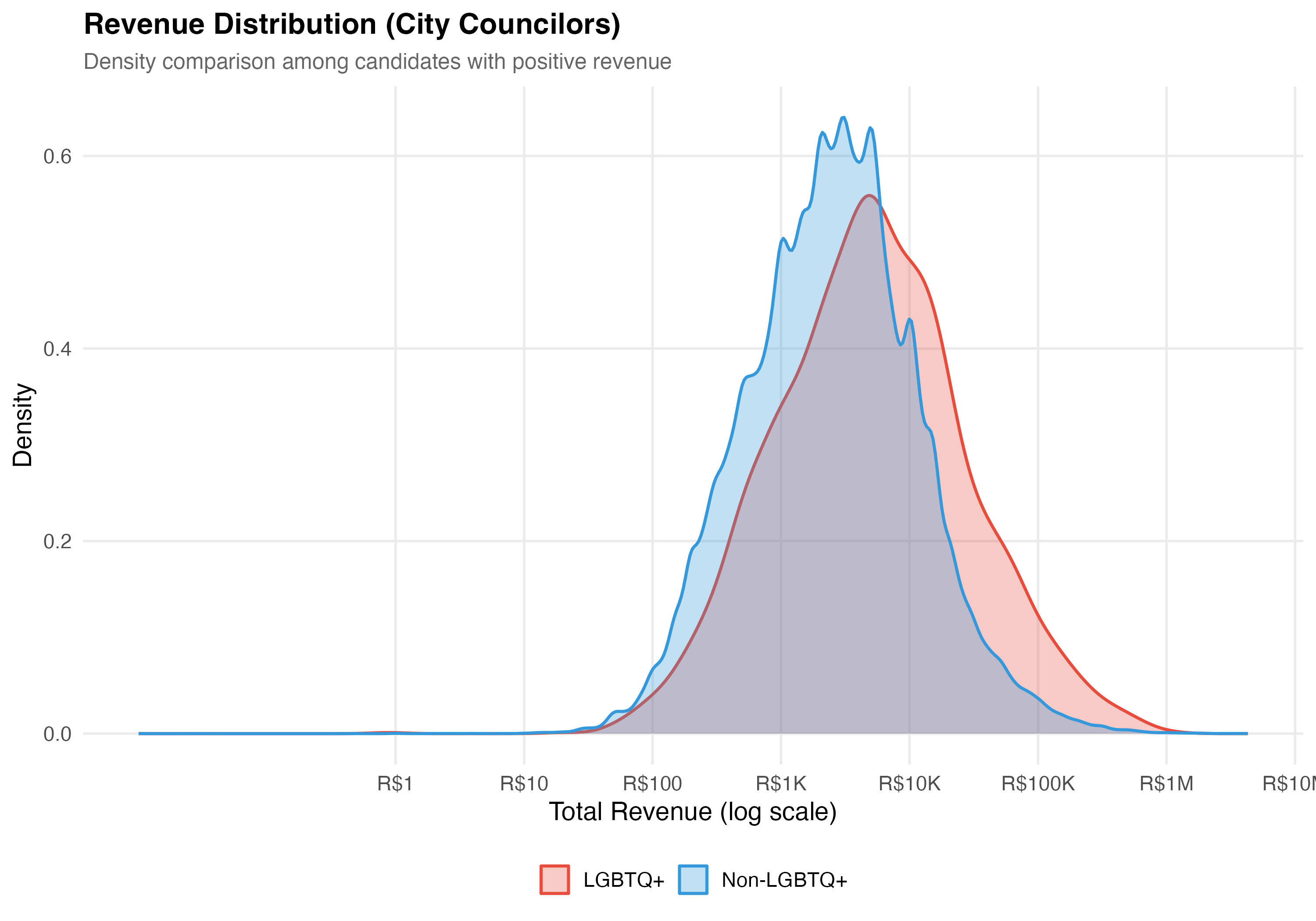
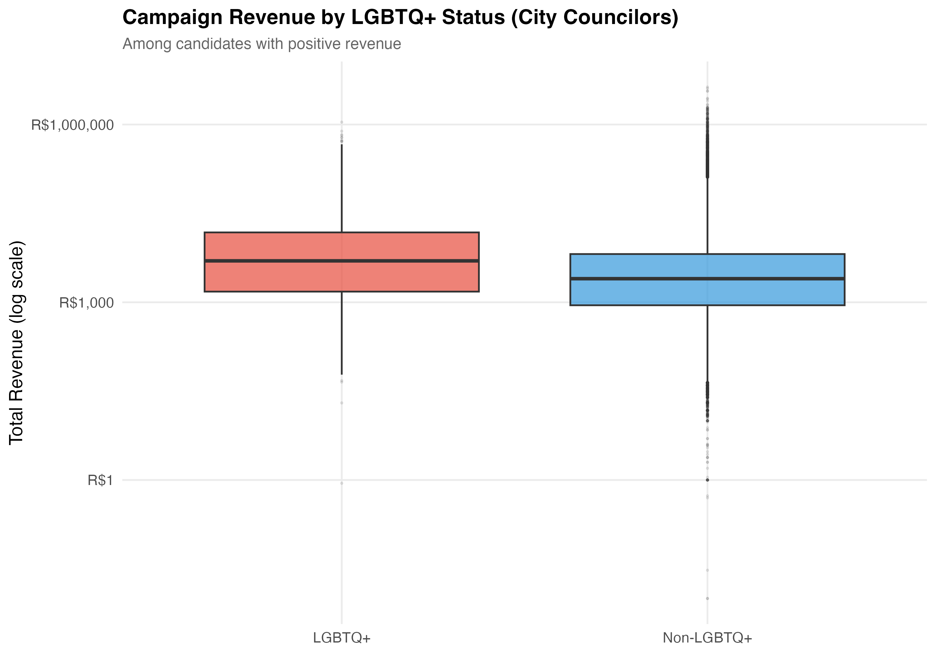
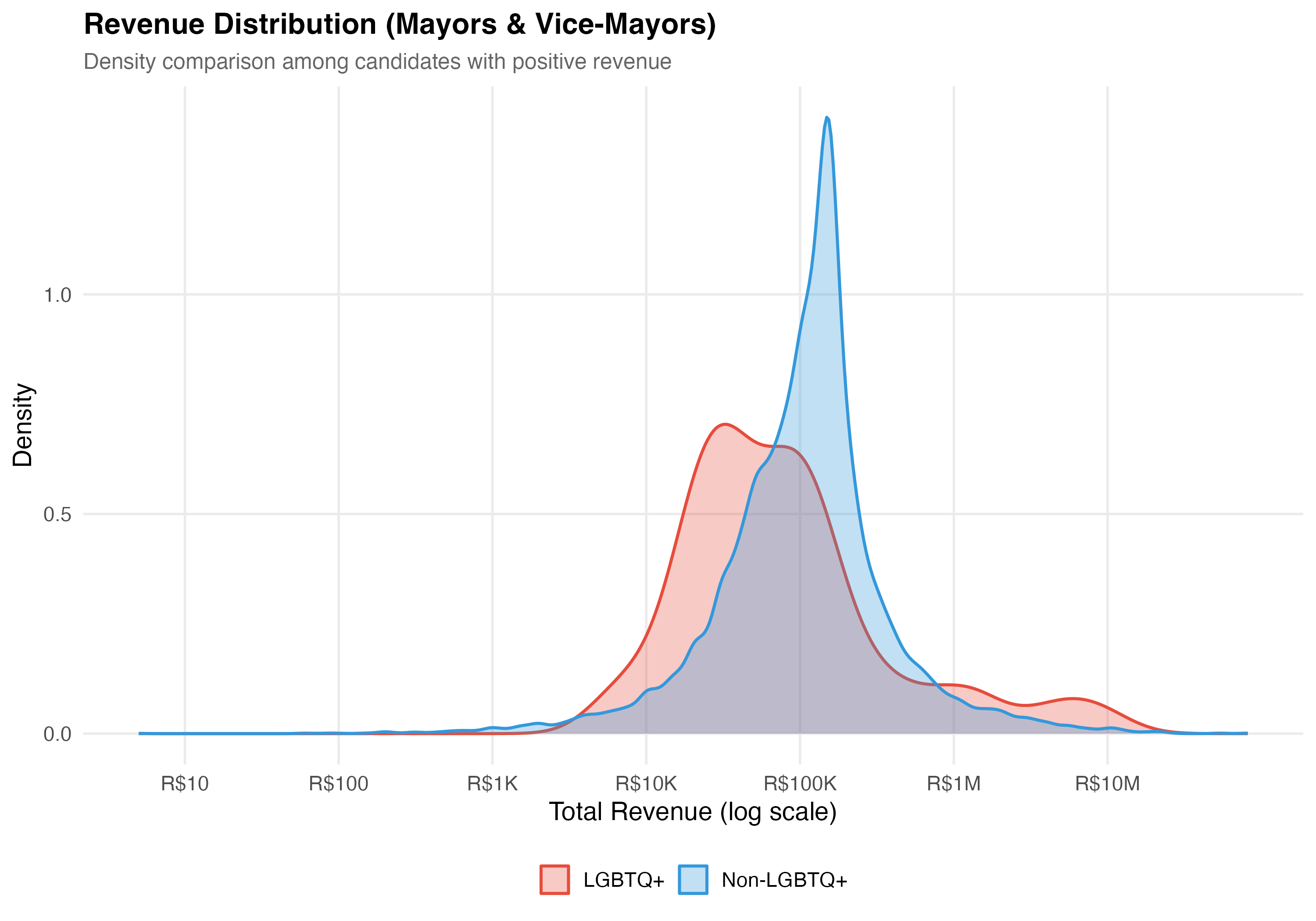
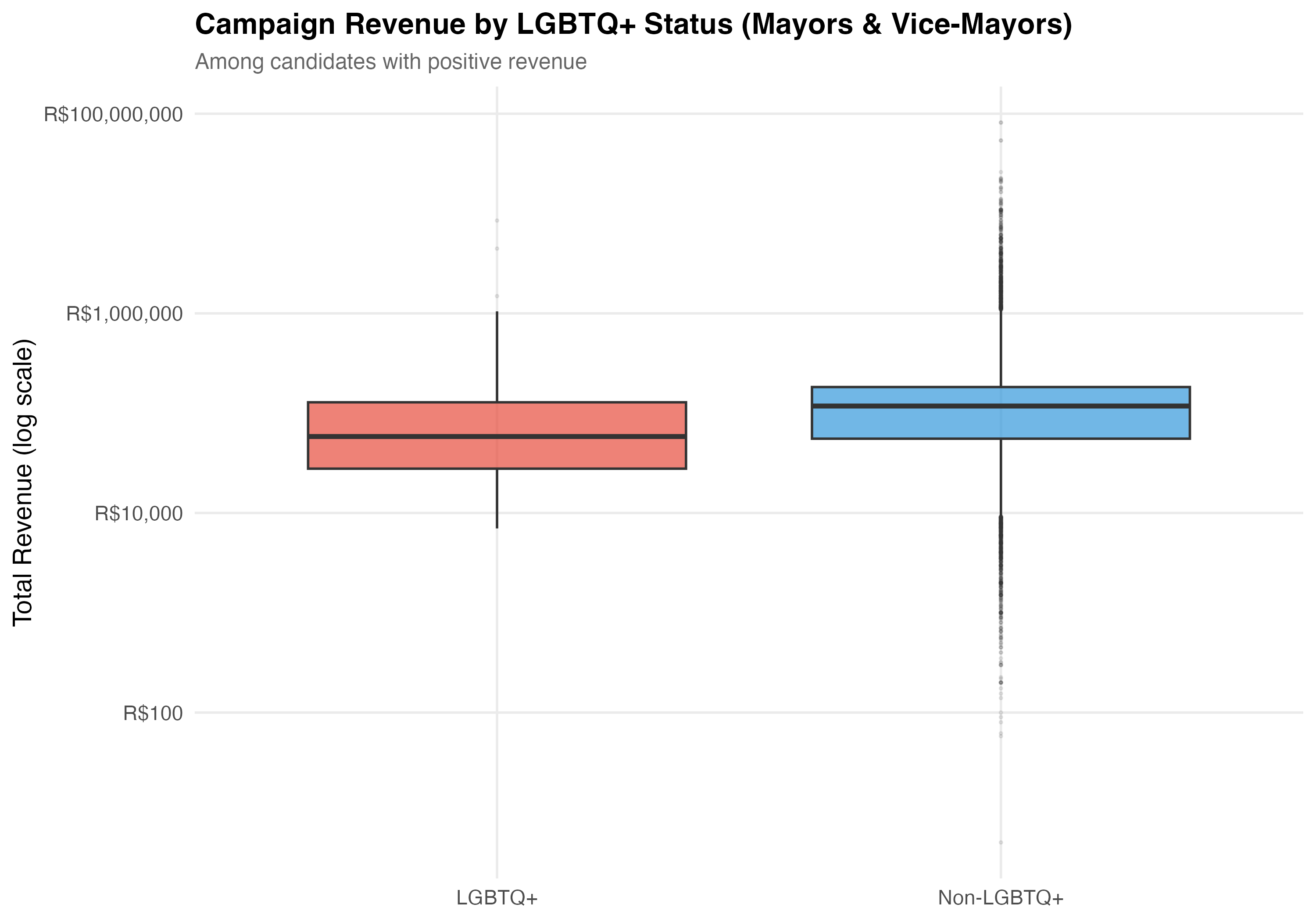
2. **LGBTQ+ revenue comparison**: LGBTQ+ candidates have a median revenue of `r format_brl(lgbtq_median)`, which is `r median_direction` than the non-LGBTQ+ median of `r format_brl(nonlgbtq_median)` (ratio: `r sprintf("%.2f", median_ratio_overall)`). At the mean, LGBTQ+ candidates raise `r format_brl(lgbtq_mean)` versus `r format_brl(nonlgbtq_mean)` (ratio: `r sprintf("%.2f", mean_ratio_overall)`).
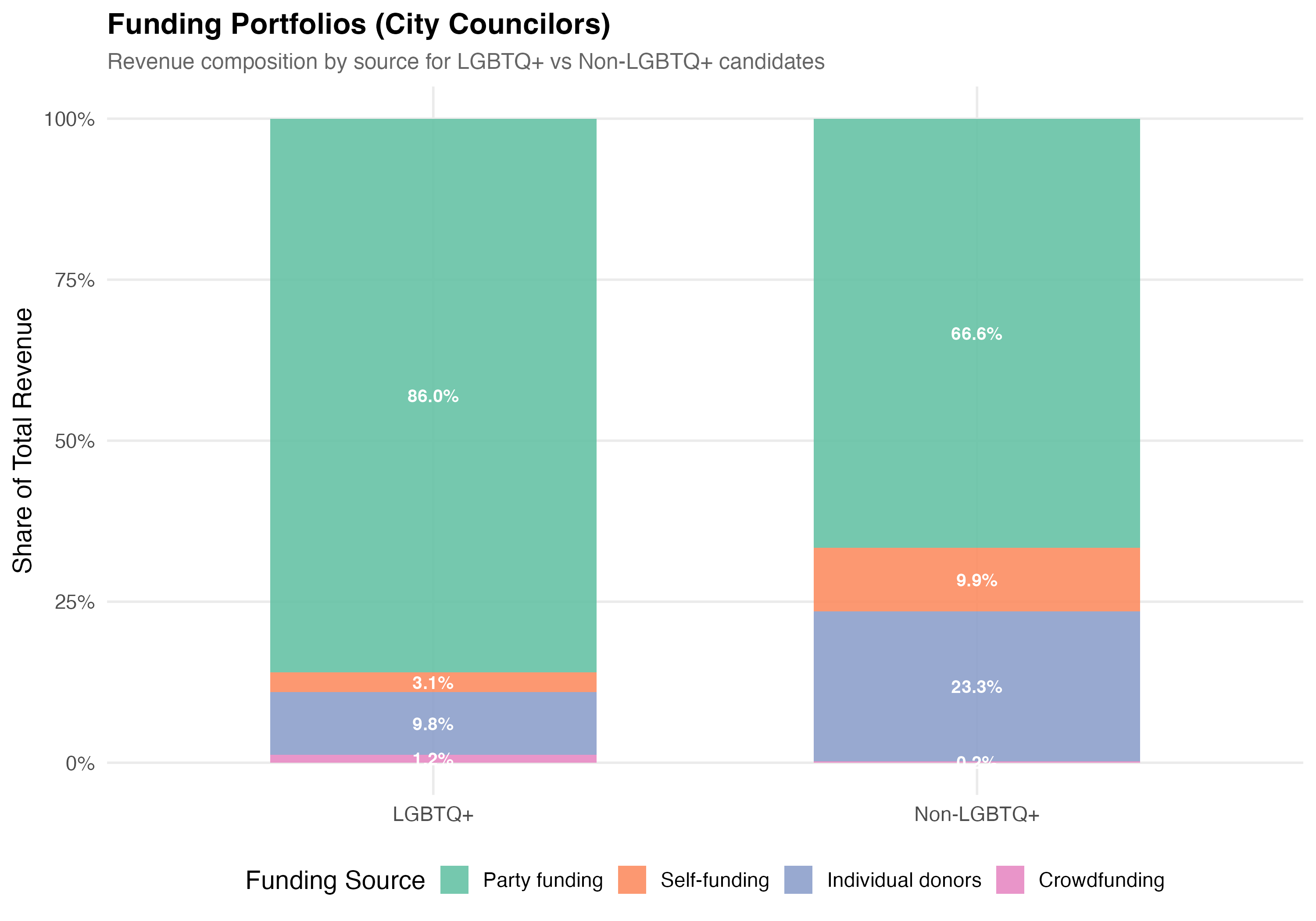
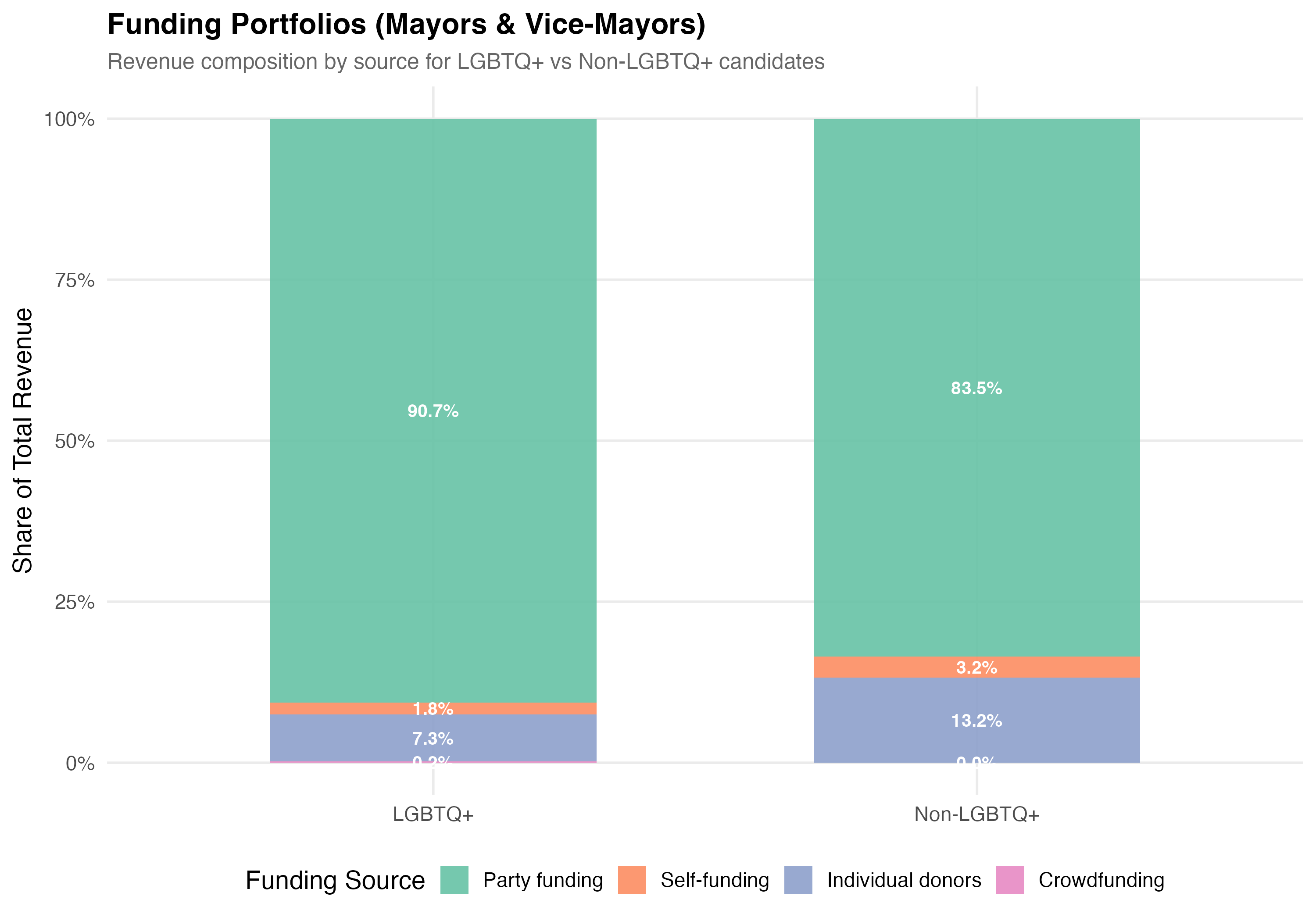
3. **Funding composition**: LGBTQ+ candidates have a `r party_diff_direction` average party funding share (`r format_pct100(lgbtq_pct_party)` vs `r format_pct100(nonlgbtq_pct_party)`) and a `r indiv_diff_direction` average individual donor share (`r format_pct100(lgbtq_pct_individual)` vs `r format_pct100(nonlgbtq_pct_individual)`) compared to non-LGBTQ+ candidates.
4. **Within-ideology patterns**: Of `r n_ideo_total` ideological blocs examined, `r n_ideo_below1_mean` show a mean revenue ratio below 1 (LGBTQ+ candidates raising less than ideological peers) and `r n_ideo_above1_mean` show a ratio above 1.
5. **Identity-specific patterns**: Across `r n_identity_cats` identity categories, `r top_median_cat` candidates have the highest median revenue (`r format_brl(top_median_val)`) and `r bottom_median_cat` candidates the lowest (`r format_brl(bottom_median_val)`). `r top_party_cat` candidates rely most heavily on party funding (`r format_pct100(top_party_val)` of revenue on average).
The next chapters examine intersectional patterns and geographic variation.