---
title: "6. Intersectional Patterns"
subtitle: "How LGBTQ+ Status Interacts with Gender, Race, and Ideology"
---
```{r setup}
source(here::here("code", "00_setup.R"))
df <- readRDS(paths$analysis_full_rds)

# Set ideology category ordering: Left → Center → Right
# Create three-way group for Trans vs LGB vs Non-LGBTQ+ comparison
df <- df %>%
  mutate(
    ideology_category = factor(ideology_category, levels = ideology_levels),
    threeway_group = case_when(
      trans_candidate ~ "Trans",
      lgb_candidate   ~ "LGB",
      TRUE            ~ "Non-LGBTQ+"
    ) %>% factor(levels = c("Non-LGBTQ+", "LGB", "Trans"))
  )
```
# Overview
LGBTQ+ candidates are not a monolith. Their experiences are shaped by other dimensions of identity --- gender, race, and the ideological environment they compete in. An intersectional lens reveals how these dimensions compound or mitigate the challenges LGBTQ+ candidates face.
This chapter systematically examines two-way and three-way interactions between LGBTQ+ status and gender, race, and ideology. We focus on two key outcomes: **candidacy patterns** (who runs) and **electoral success** (who wins), along with the campaign finance dimension explored in the previous chapter.
::: {.callout-note}
## Results by Position Type
Two-way intersectional analyses (LGBTQ+ x Gender, LGBTQ+ x Race, LGBTQ+ x Ideology) are presented separately for city councilors and mayors/vice-mayors. The triple intersection and trans-specific sections pool across positions because further disaggregation produces cell sizes too small for meaningful comparison.
:::
::: {.callout-note}
## Methodological Note
Intersectional analysis with small subgroup sizes must be interpreted cautiously. When cell sizes drop below 30, we flag the estimates as imprecise. For trans candidates specifically, the small N makes most intersectional breakdowns unreliable for inferential purposes --- we present them descriptively as a starting point.
:::
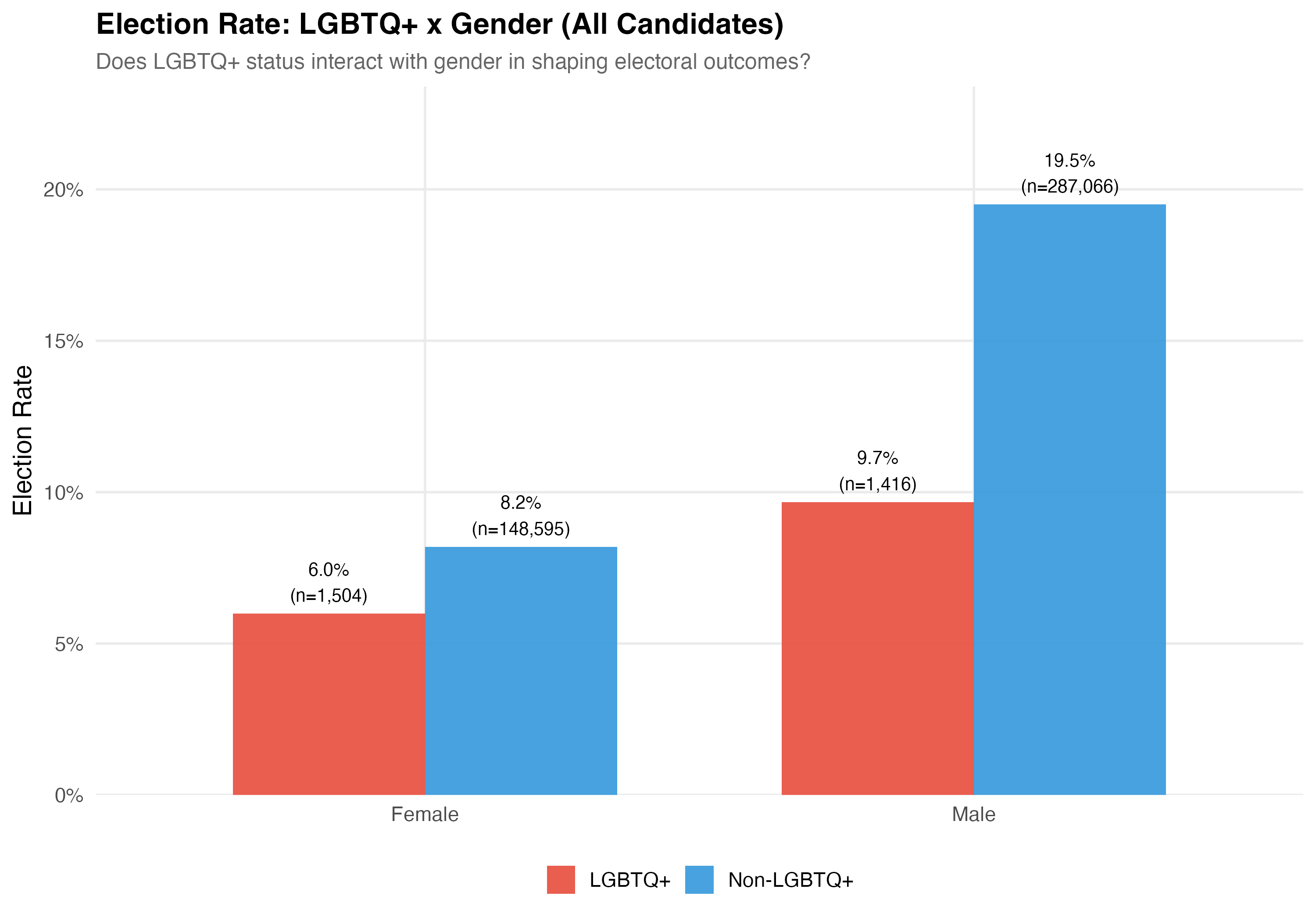
# LGBTQ+ x Gender
## Cross-Tabulation
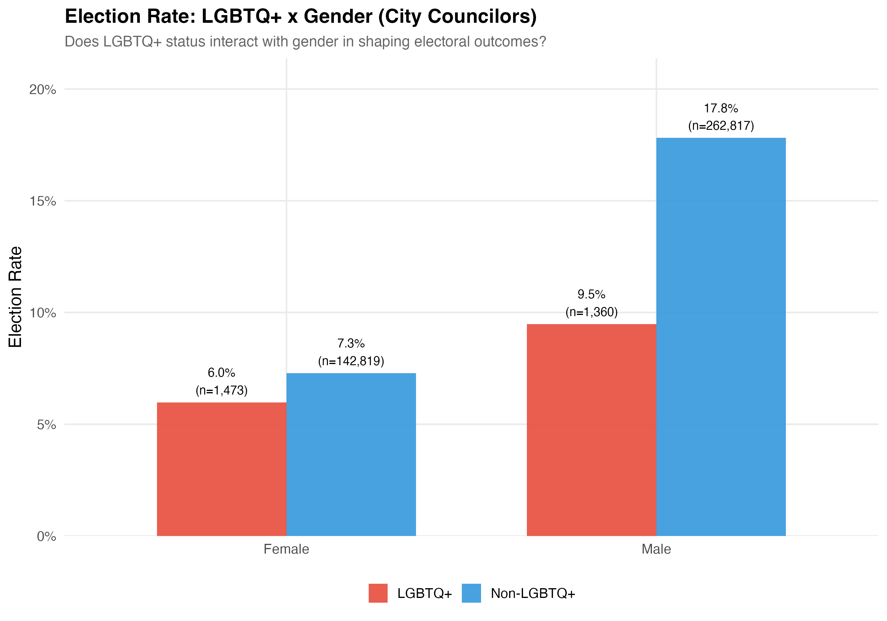
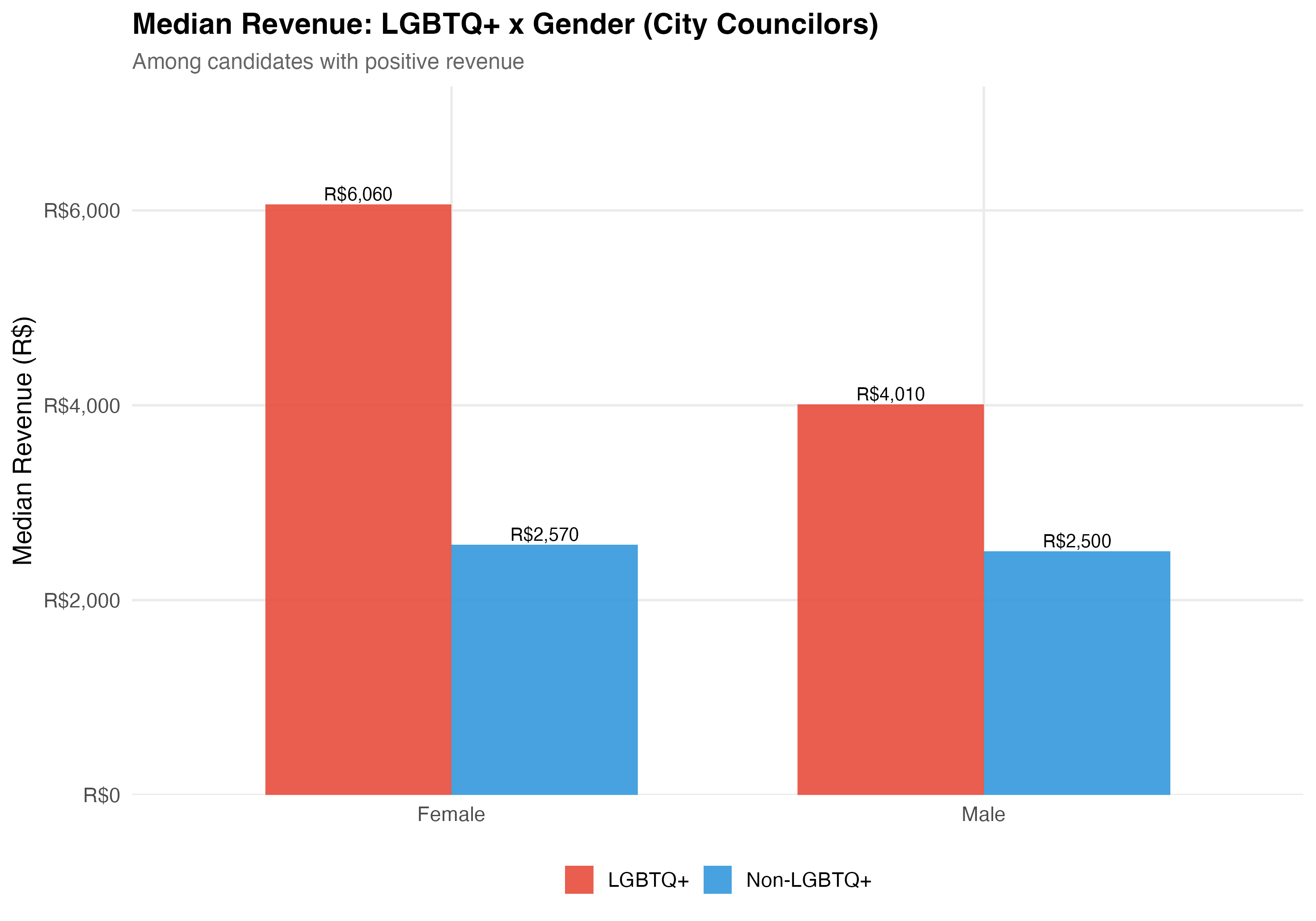
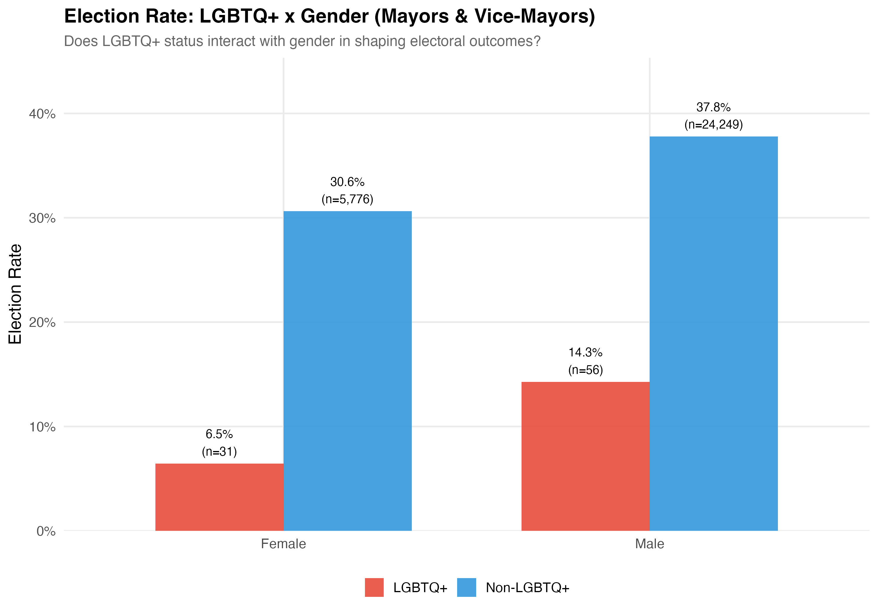
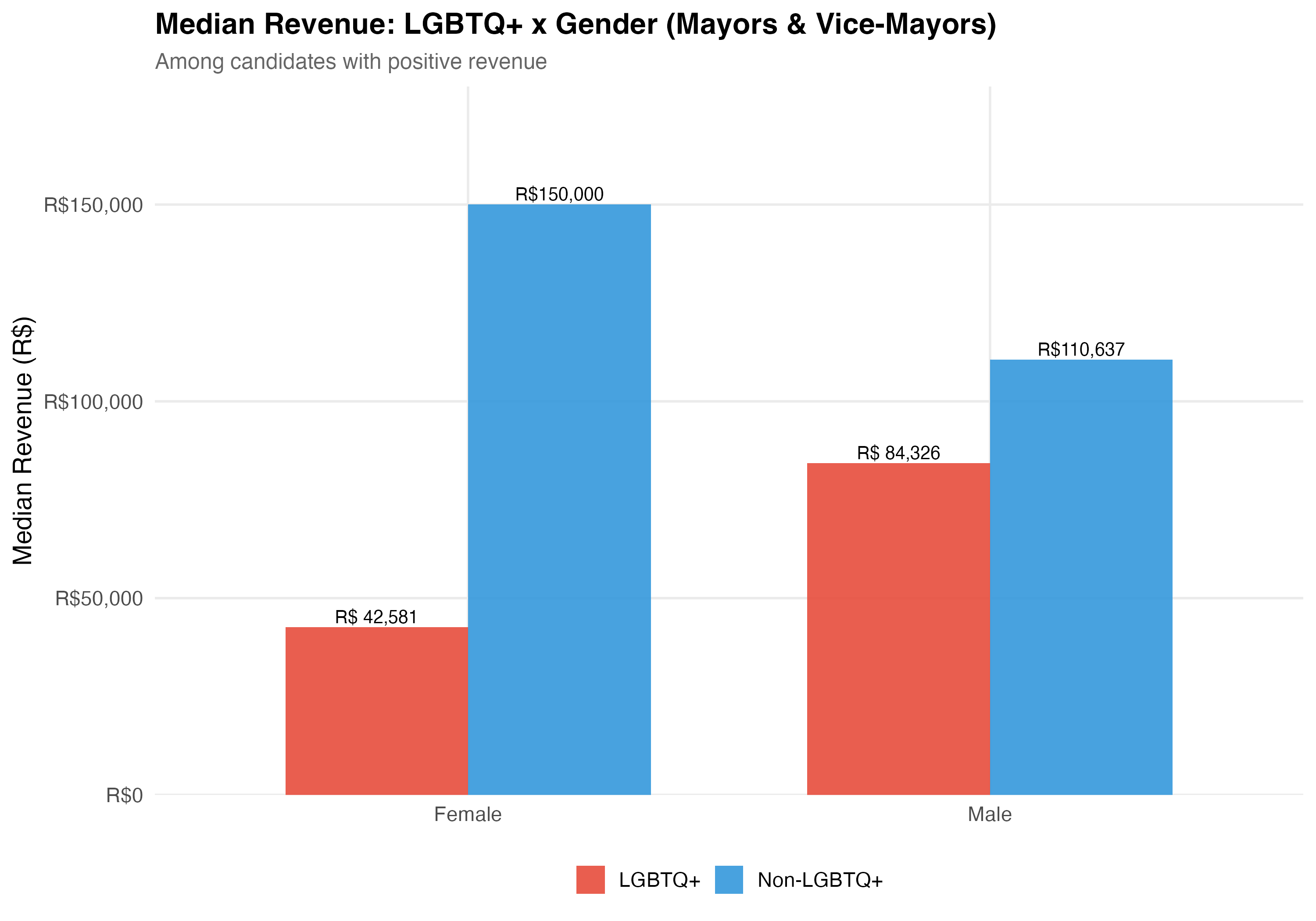
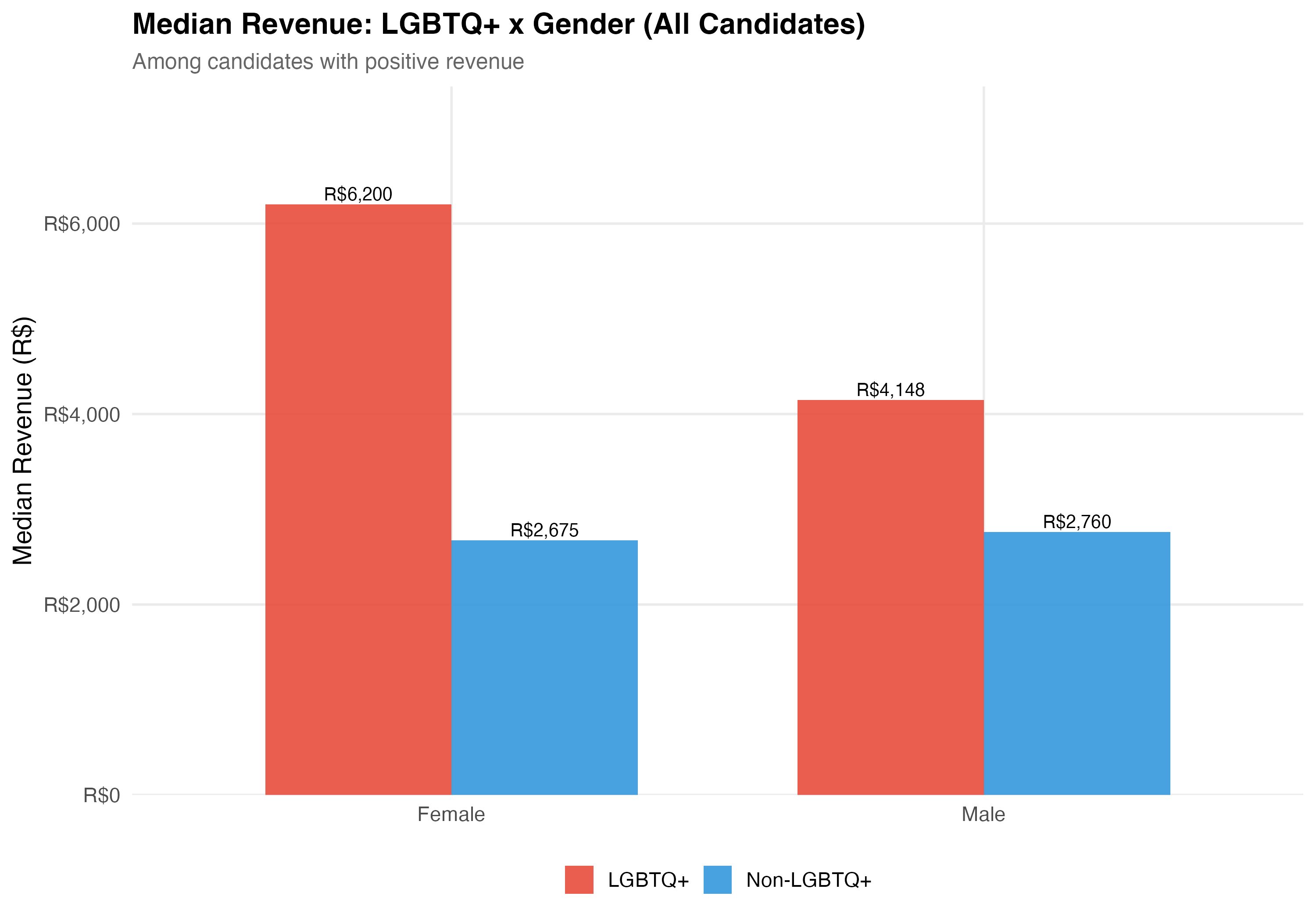
Gender is recorded on TSE registration forms (Female/Male). **Election rate** is the proportion of candidates who won their race. **Total revenue** is the sum of all campaign receipts registered with the TSE, including cash donations, party transfers, self-funding, and the estimated monetary value of in-kind contributions.
```{r gender-tabset}
#| results: asis
render_gender_intersection <- function(data, tab_name) {
  d <- data %>%
    filter(!is.na(female), !is.na(elected)) %>%
    mutate(
      lgbtq_group  = if_else(lgbtq_candidate, "LGBTQ+", "Non-LGBTQ+"),
      gender_label = if_else(female, "Female", "Male")
    )

  # --- Cross-tabulation table ---
  cat("### Cross-Tabulation\n\n")

  lgbtq_gender <- d %>%
    group_by(lgbtq_group, gender_label) %>%
    summarise(
      N             = n(),
      Elected       = sum(elected),
      `Elect. Rate` = format_pct(mean(elected)),
      `Mean Rev.`   = format_brl(mean(total_revenue, na.rm = TRUE)),
      `Median Rev.` = format_brl(median(total_revenue, na.rm = TRUE)),
      .groups = "drop"
    )

  lgbtq_gender %>%
    rename(`LGBTQ+ Status` = lgbtq_group, Gender = gender_label) %>%
    cat_kable(align = c("l", "l", "r", "r", "r", "r", "r"))

  # --- Election rate chart ---
  cat("### Election Rate\n\n")

  p_rate <- d %>%
    group_by(lgbtq_group, gender_label) %>%
    summarise(rate = mean(elected), n = n(), .groups = "drop") %>%
    ggplot(aes(x = gender_label, y = rate, fill = lgbtq_group)) +
    geom_col(position = "dodge", alpha = 0.9, width = 0.7) +
    geom_text(aes(label = paste0(format_pct(rate), "\n(n=", format_n(n), ")")),
              position = position_dodge(width = 0.7), vjust = -0.3, size = 3.5) +
    scale_fill_manual(values = pal_lgbtq, name = NULL) +
    scale_y_continuous(labels = percent, expand = expansion(mult = c(0, 0.2))) +
    labs(
      x     = NULL, y = "Election Rate",
      title = paste0("Election Rate: LGBTQ+ x Gender (", tab_name, ")"),
      subtitle = "Does LGBTQ+ status interact with gender in shaping electoral outcomes?"
    )
  cat_plot(p_rate, paste0("06-lgbtq-gender-rate-", pos_suffix(tab_name)))

  # --- Revenue chart ---
  cat("### Median Revenue\n\n")

  rev_data <- data %>%
    filter(!is.na(female), total_revenue > 0) %>%
    mutate(
      lgbtq_group  = if_else(lgbtq_candidate, "LGBTQ+", "Non-LGBTQ+"),
      gender_label = if_else(female, "Female", "Male")
    ) %>%
    group_by(lgbtq_group, gender_label) %>%
    summarise(median_rev = median(total_revenue), n = n(), .groups = "drop")

  p_rev <- rev_data %>%
    ggplot(aes(x = gender_label, y = median_rev, fill = lgbtq_group)) +
    geom_col(position = "dodge", alpha = 0.9, width = 0.7) +
    geom_text(aes(label = format_brl(median_rev)),
              position = position_dodge(width = 0.7), vjust = -0.3, size = 3.5) +
    scale_fill_manual(values = pal_lgbtq, name = NULL) +
    scale_y_continuous(labels = label_dollar(prefix = "R$", big.mark = ","),
                       expand = expansion(mult = c(0, 0.2))) +
    labs(
      x     = NULL, y = "Median Revenue (R$)",
      title = paste0("Median Revenue: LGBTQ+ x Gender (", tab_name, ")"),
      subtitle = "Among candidates with positive revenue"
    )
  cat_plot(p_rev, paste0("06-lgbtq-gender-revenue-", pos_suffix(tab_name)))

  cat("::: {.callout-important}\n")
  cat("## Double Disadvantage?\n")
  cat("The \"double disadvantage\" hypothesis predicts that marginalized identities compound ",
      "rather than substitute for each other --- so LGBTQ+ women would face the lowest ",
      "election rates and revenue. The data above allow us to assess whether this pattern holds.\n")
  cat(":::\n\n")
}

render_position_tabset(render_gender_intersection, df)
```
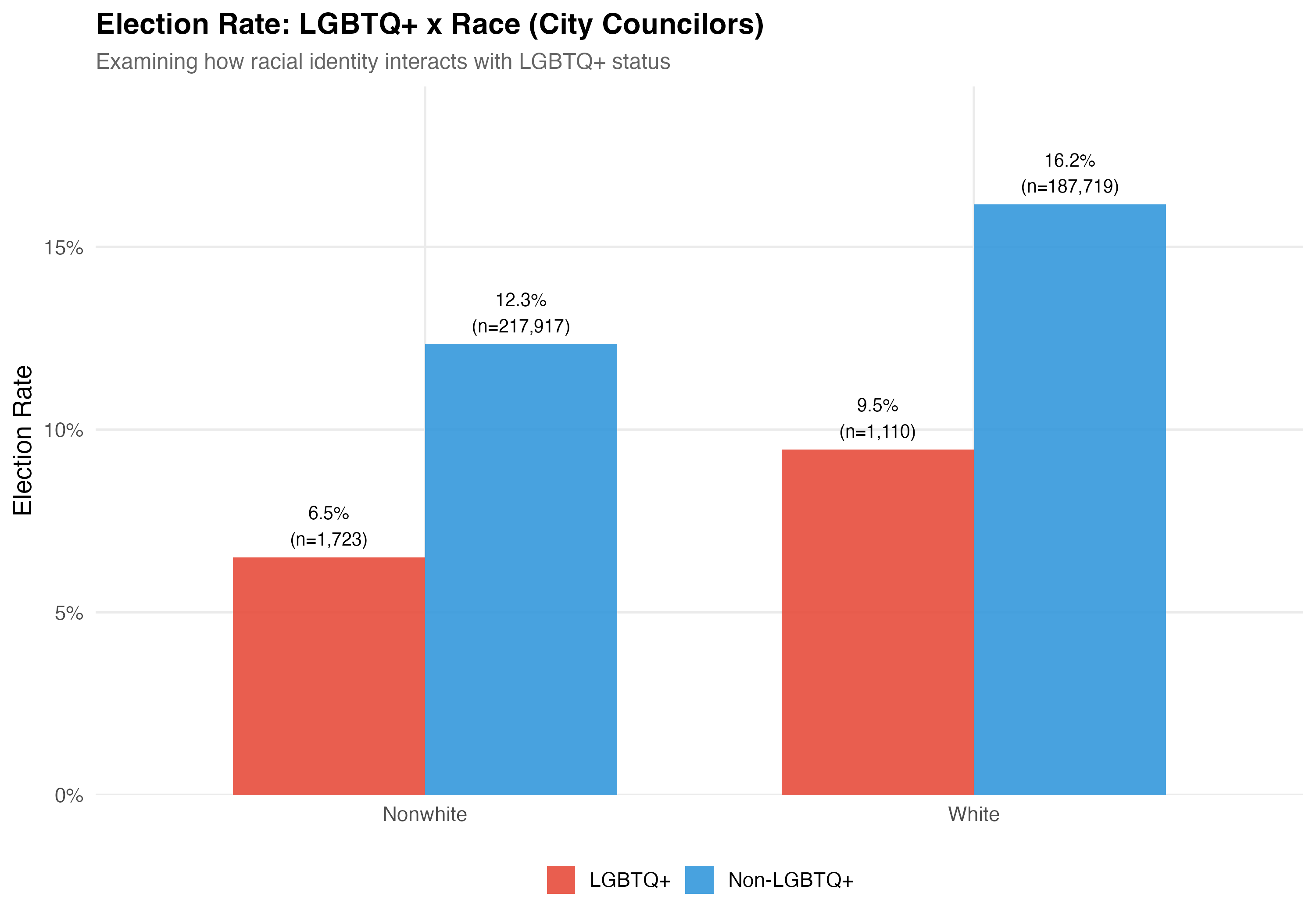
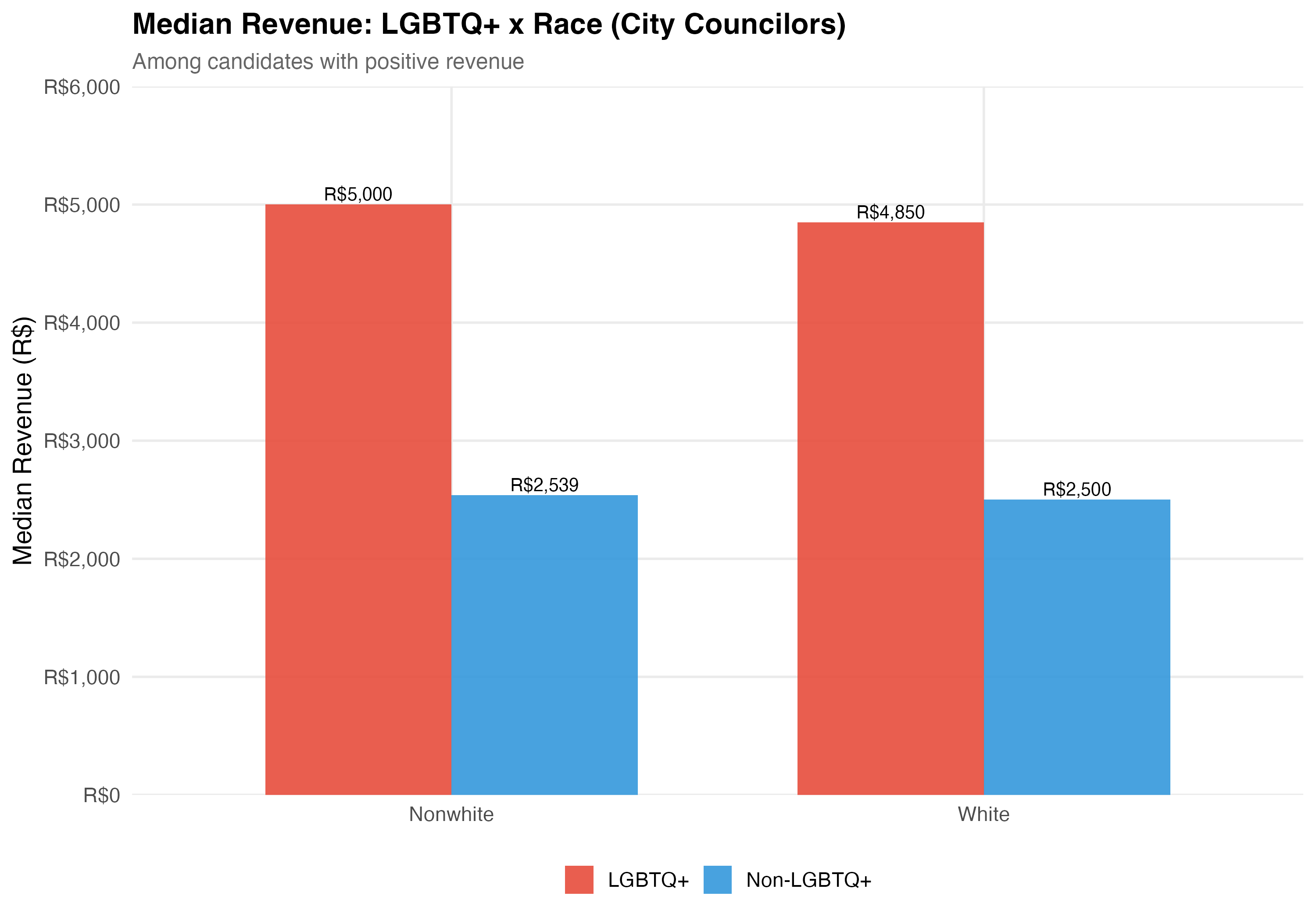
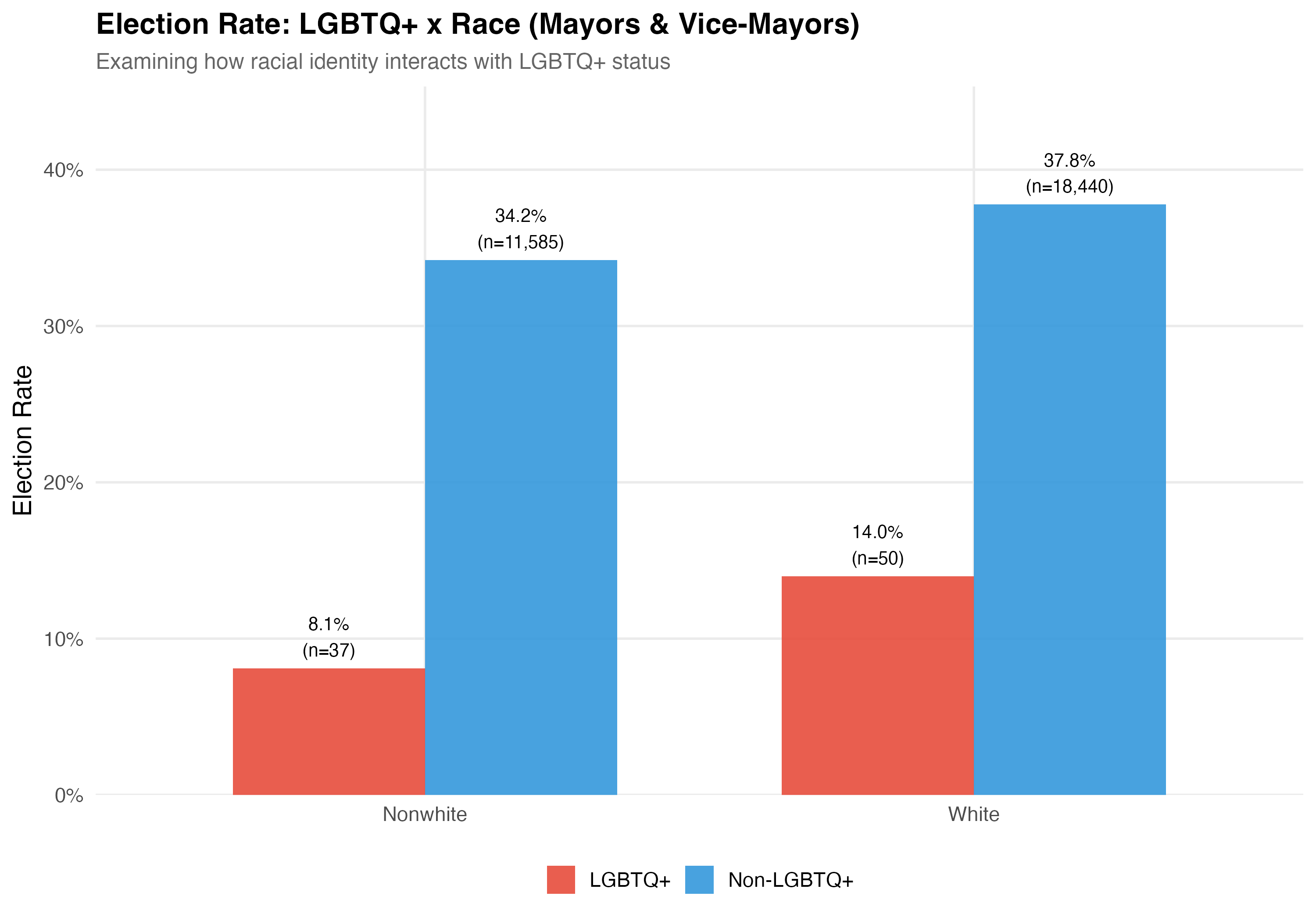
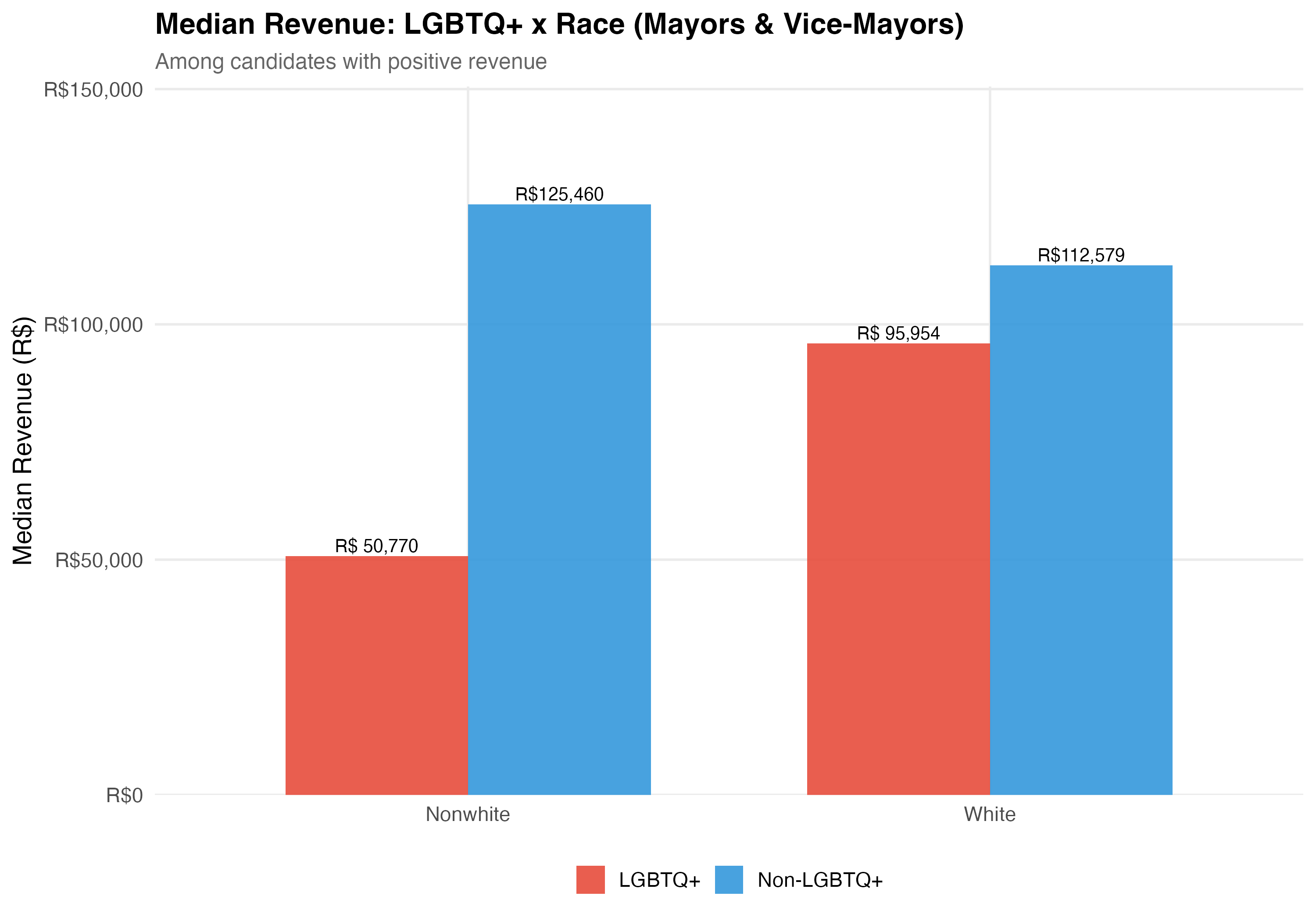
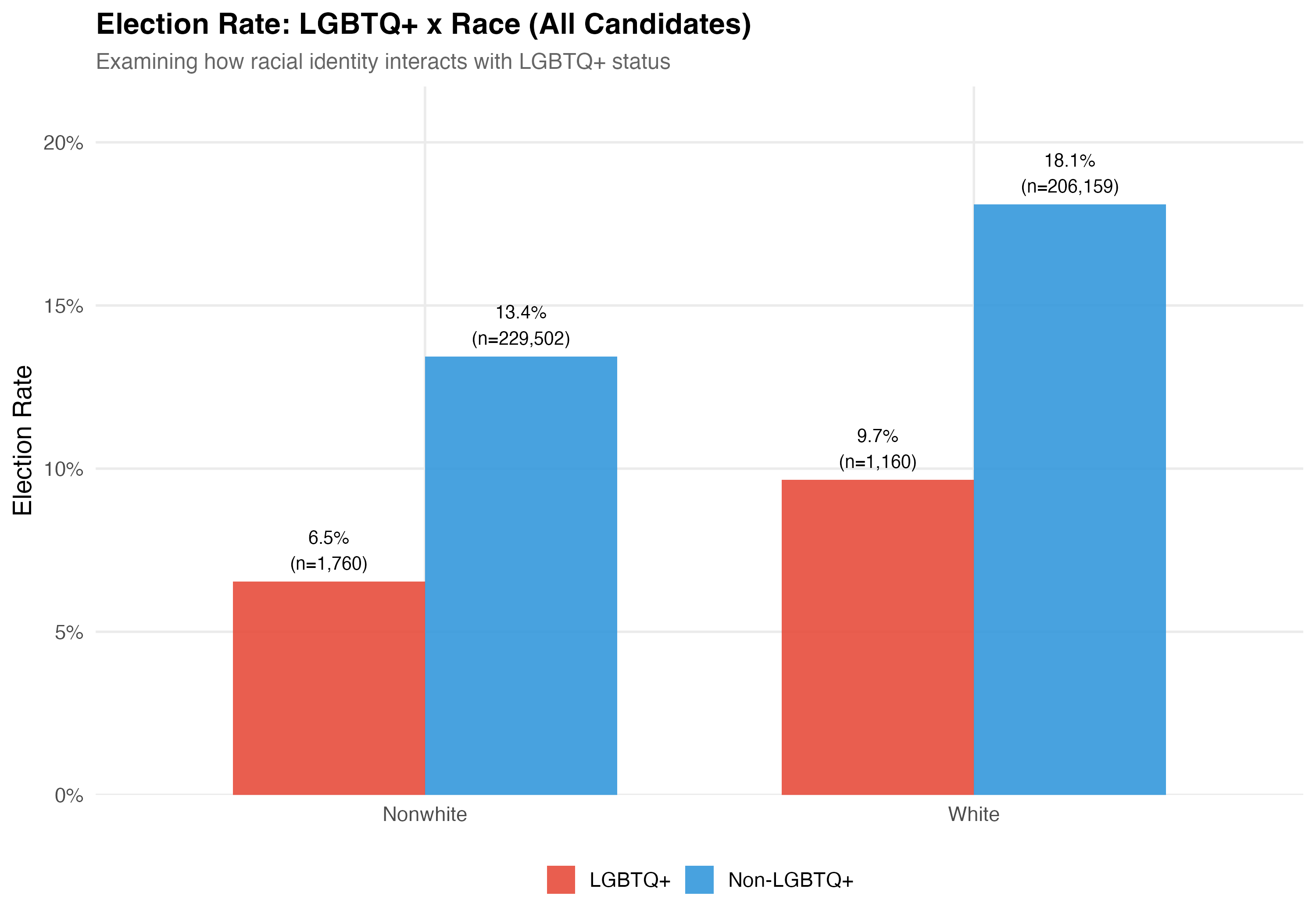
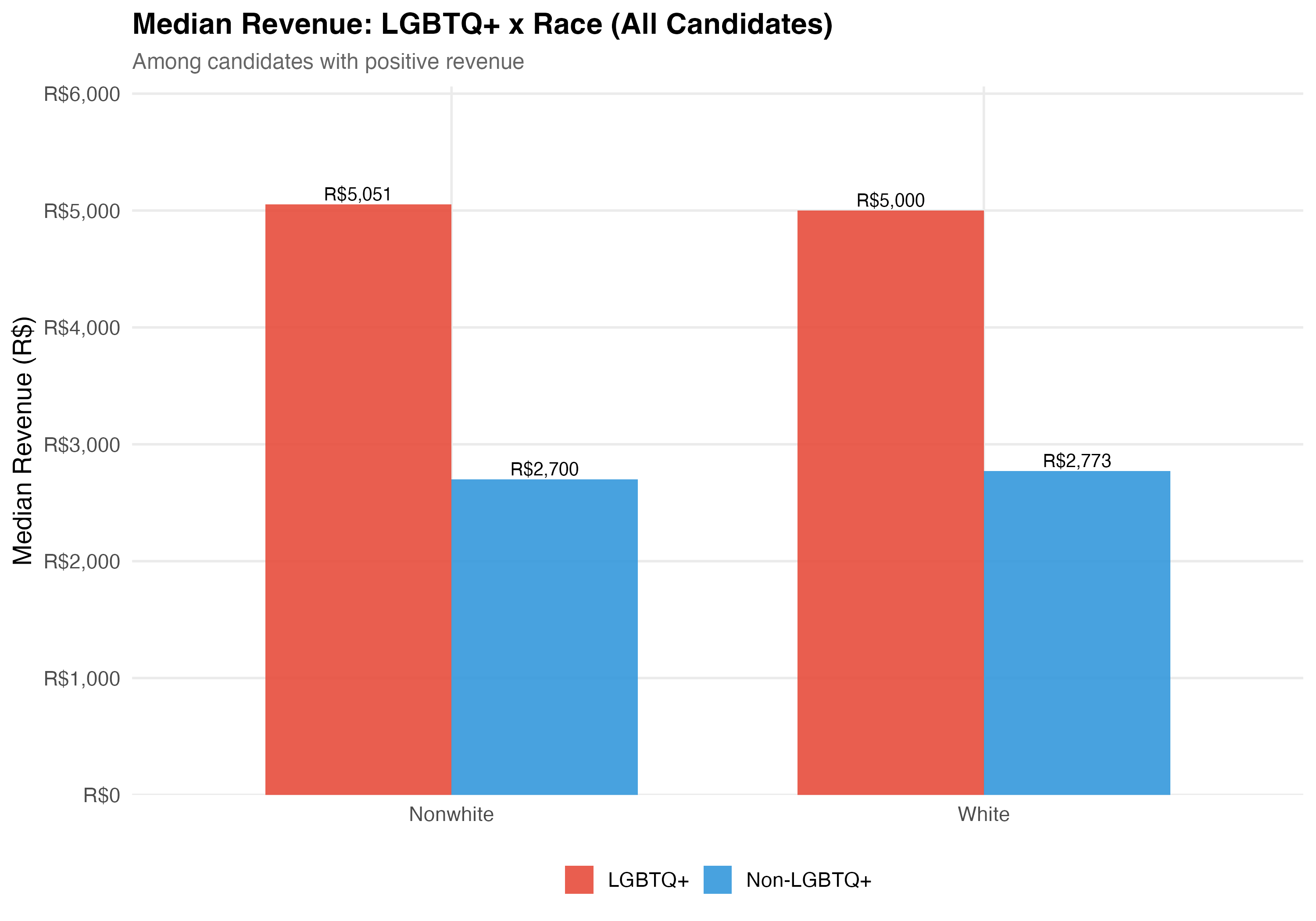
# LGBTQ+ x Race
## Cross-Tabulation
Race is simplified into White and Nonwhite (Black, Brown, and Other combined) for the intersectional analysis.
```{r race-tabset}
#| results: asis
render_race_intersection <- function(data, tab_name) {
  d <- data %>%
    filter(!is.na(nonwhite), !is.na(elected)) %>%
    mutate(
      lgbtq_group = if_else(lgbtq_candidate, "LGBTQ+", "Non-LGBTQ+"),
      race_label  = if_else(nonwhite, "Nonwhite", "White")
    )

  # --- Cross-tabulation table ---
  cat("### Cross-Tabulation\n\n")

  lgbtq_race <- d %>%
    group_by(lgbtq_group, race_label) %>%
    summarise(
      N             = n(),
      Elected       = sum(elected),
      `Elect. Rate` = format_pct(mean(elected)),
      `Mean Rev.`   = format_brl(mean(total_revenue, na.rm = TRUE)),
      `Median Rev.` = format_brl(median(total_revenue, na.rm = TRUE)),
      .groups = "drop"
    )

  lgbtq_race %>%
    rename(`LGBTQ+ Status` = lgbtq_group, Race = race_label) %>%
    cat_kable(align = c("l", "l", "r", "r", "r", "r", "r"))

  # --- Election rate chart ---
  cat("### Election Rate\n\n")

  p_rate <- d %>%
    group_by(lgbtq_group, race_label) %>%
    summarise(rate = mean(elected), n = n(), .groups = "drop") %>%
    ggplot(aes(x = race_label, y = rate, fill = lgbtq_group)) +
    geom_col(position = "dodge", alpha = 0.9, width = 0.7) +
    geom_text(aes(label = paste0(format_pct(rate), "\n(n=", format_n(n), ")")),
              position = position_dodge(width = 0.7), vjust = -0.3, size = 3.5) +
    scale_fill_manual(values = pal_lgbtq, name = NULL) +
    scale_y_continuous(labels = percent, expand = expansion(mult = c(0, 0.2))) +
    labs(
      x     = NULL, y = "Election Rate",
      title = paste0("Election Rate: LGBTQ+ x Race (", tab_name, ")"),
      subtitle = "Examining how racial identity interacts with LGBTQ+ status"
    )
  cat_plot(p_rate, paste0("06-lgbtq-race-rate-", pos_suffix(tab_name)))

  # --- Revenue chart ---
  cat("### Median Revenue\n\n")

  rev_data <- data %>%
    filter(!is.na(nonwhite), total_revenue > 0) %>%
    mutate(
      lgbtq_group = if_else(lgbtq_candidate, "LGBTQ+", "Non-LGBTQ+"),
      race_label  = if_else(nonwhite, "Nonwhite", "White")
    ) %>%
    group_by(lgbtq_group, race_label) %>%
    summarise(median_rev = median(total_revenue), n = n(), .groups = "drop")

  p_rev <- rev_data %>%
    ggplot(aes(x = race_label, y = median_rev, fill = lgbtq_group)) +
    geom_col(position = "dodge", alpha = 0.9, width = 0.7) +
    geom_text(aes(label = format_brl(median_rev)),
              position = position_dodge(width = 0.7), vjust = -0.3, size = 3.5) +
    scale_fill_manual(values = pal_lgbtq, name = NULL) +
    scale_y_continuous(labels = label_dollar(prefix = "R$", big.mark = ","),
                       expand = expansion(mult = c(0, 0.2))) +
    labs(
      x     = NULL, y = "Median Revenue (R$)",
      title = paste0("Median Revenue: LGBTQ+ x Race (", tab_name, ")"),
      subtitle = "Among candidates with positive revenue"
    )
  cat_plot(p_rev, paste0("06-lgbtq-race-revenue-", pos_suffix(tab_name)))
}

render_position_tabset(render_race_intersection, df)
```
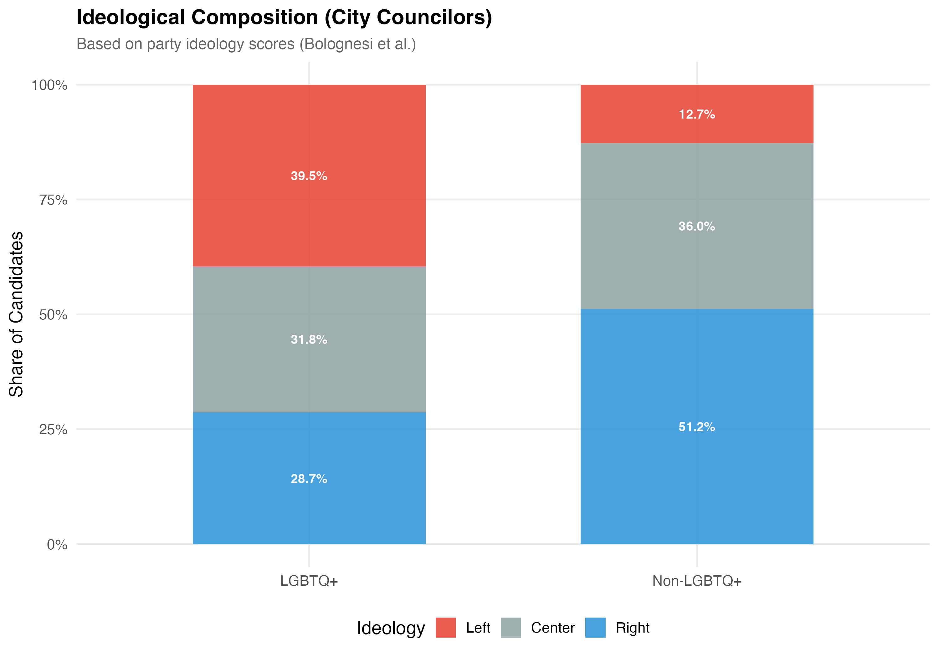
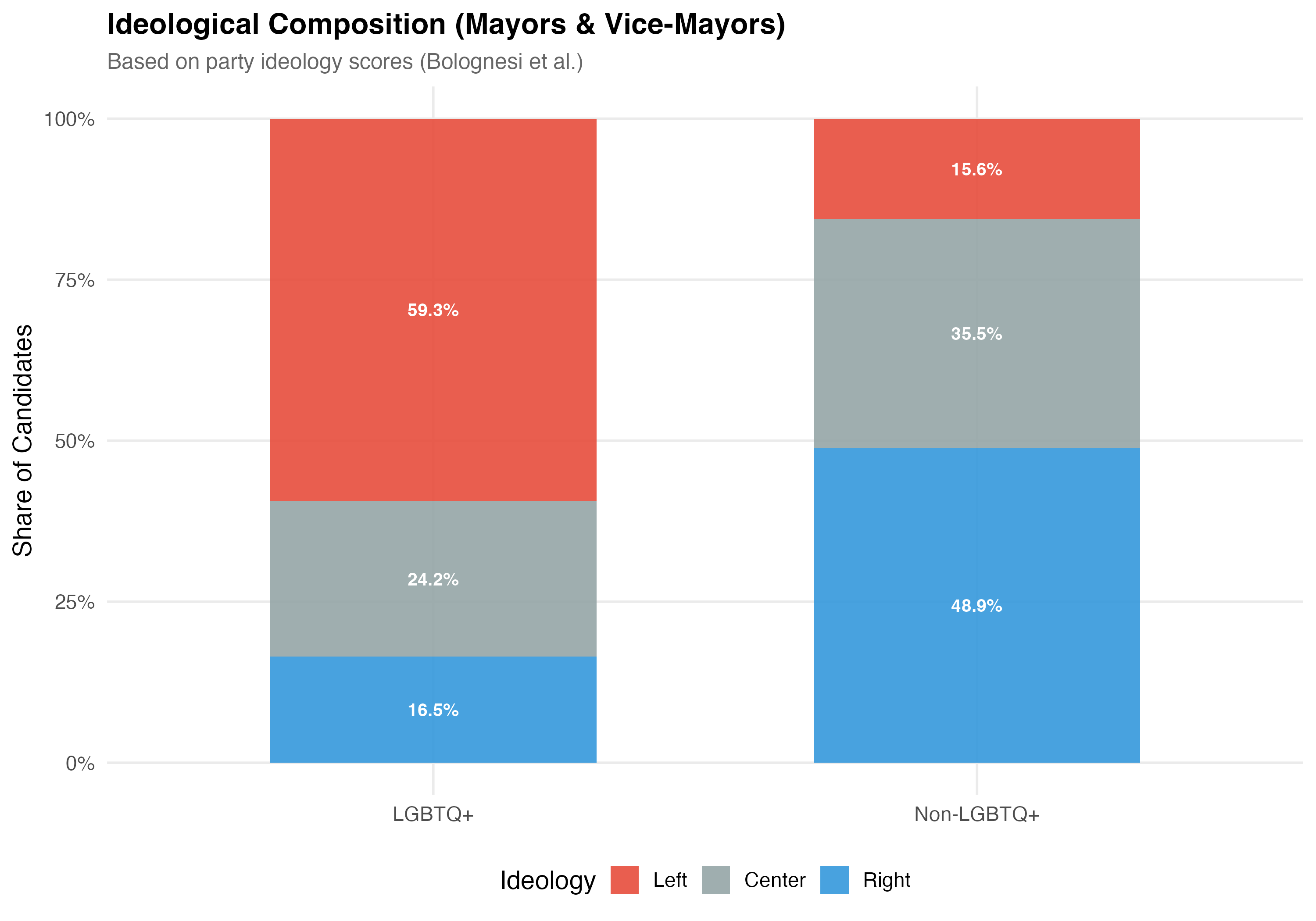
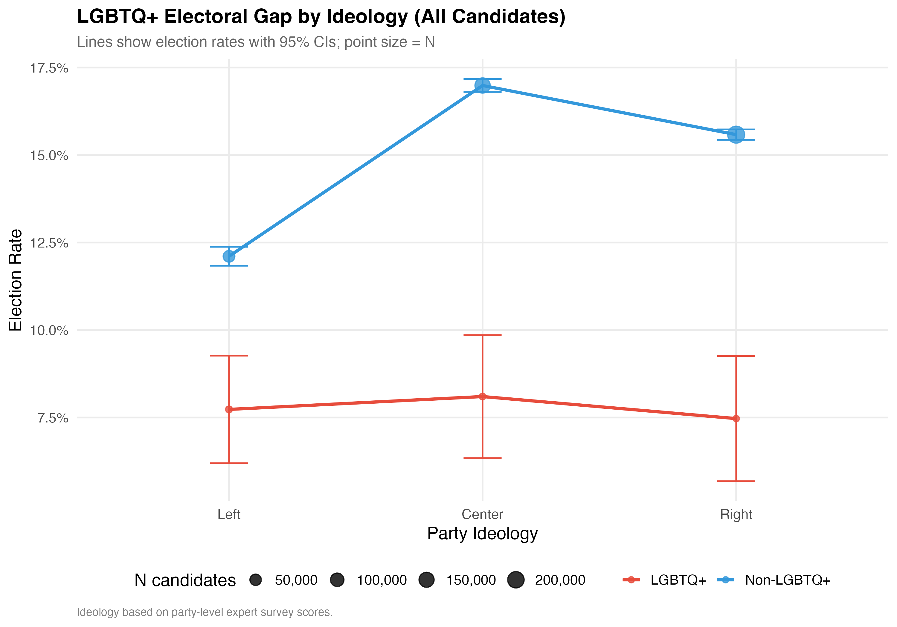
# LGBTQ+ x Ideology
## Distribution Across the Ideological Spectrum
Party ideology scores are drawn from Bolognesi et al.'s expert survey (0--10 left-right scale; Left < 4.0, Center 4.0--7.1, Right > 7.1).
```{r ideology-tabset}
#| results: asis
render_ideology_intersection <- function(data, tab_name) {
simplified <- use_simplified(data)
# --- Ideology distribution ---
cat("### Ideological Composition\n\n")
p_mosaic <- data %>%
filter(!is.na(ideology_category)) %>%
mutate(lgbtq_group = if_else(lgbtq_candidate, "LGBTQ+", "Non-LGBTQ+")) %>%
count(lgbtq_group, ideology_category) %>%
group_by(lgbtq_group) %>%
mutate(pct = n / sum(n)) %>%
ungroup() %>%
ggplot(aes(x = lgbtq_group, y = pct, fill = ideology_category)) +
geom_col(alpha = 0.9, width = 0.6) +
geom_text(aes(label = format_pct(pct)),
position = position_stack(vjust = 0.5), size = 3.5, color = "white",
fontface = "bold") +
scale_fill_manual(values = pal_ideology, name = "Ideology") +
scale_y_continuous(labels = percent) +
labs(
x = NULL, y = "Share of Candidates",
title = paste0("Ideological Composition (", tab_name, ")"),
subtitle = "Based on party ideology scores (Bolognesi et al.)"
)
cat_plot(p_mosaic, paste0("06-lgbtq-ideology-mosaic-", pos_suffix(tab_name)))
# --- Election rates by ideology ---
cat("### Election Rates by Ideology\n\n")
d_ideo <- data %>%
filter(!is.na(ideology_category), !is.na(elected)) %>%
mutate(lgbtq_group = if_else(lgbtq_candidate, "LGBTQ+", "Non-LGBTQ+"))
ideo_rates <- d_ideo %>%
group_by(ideology_category, lgbtq_group) %>%
summarise(N = n(), Rate = format_pct(mean(elected)), .groups = "drop") %>%
pivot_wider(names_from = lgbtq_group, values_from = c(N, Rate)) %>%
select(
Ideology = ideology_category,
`N LGBTQ+` = `N_LGBTQ+`,
`N Non-LGBTQ+` = `N_Non-LGBTQ+`,
`Rate LGBTQ+` = `Rate_LGBTQ+`,
`Rate Non-LGBTQ+` = `Rate_Non-LGBTQ+`
)
cat_kable(ideo_rates, align = c("l", "r", "r", "r", "r"))
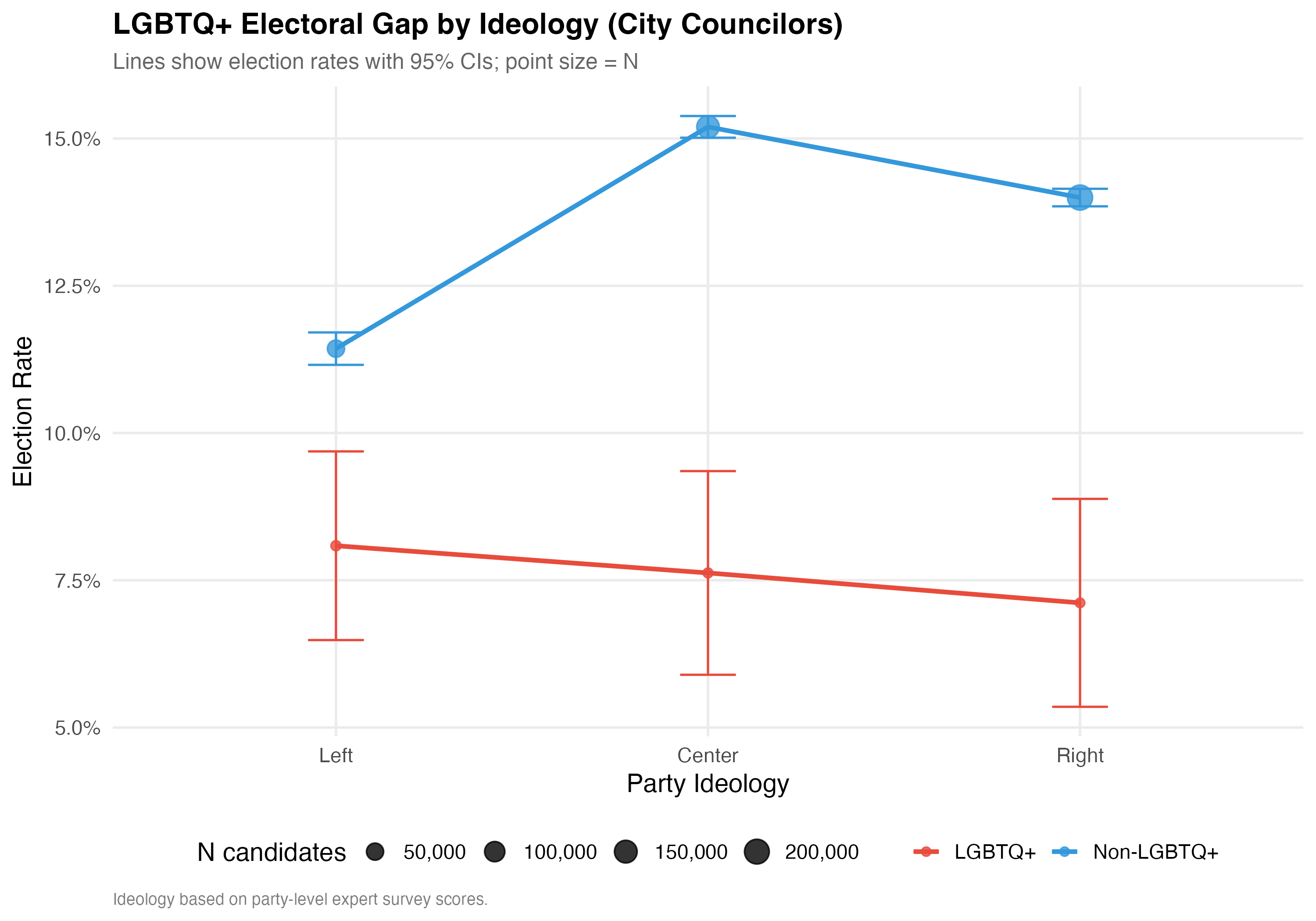
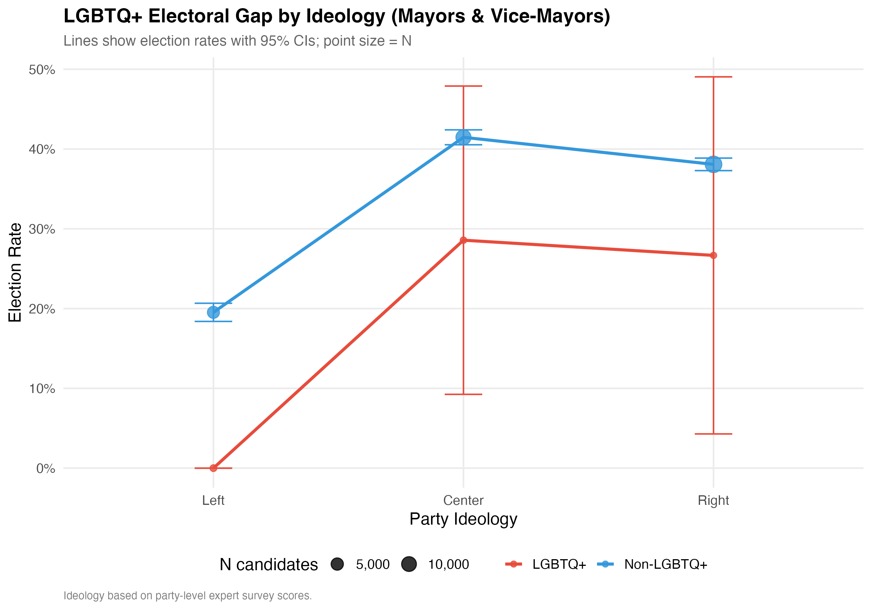
# --- Interaction plot ---
cat("### Interaction Plot\n\n")
p_interaction <- d_ideo %>%
group_by(ideology_category, lgbtq_group) %>%
summarise(
rate = mean(elected), n = n(),
se = sqrt(rate * (1 - rate) / n),
.groups = "drop"
) %>%
ggplot(aes(x = ideology_category, y = rate,
color = lgbtq_group, group = lgbtq_group)) +
geom_line(linewidth = 1.2) +
geom_point(aes(size = n), alpha = 0.8) +
geom_errorbar(aes(ymin = pmax(rate - 1.96 * se, 0),
ymax = pmin(rate + 1.96 * se, 1)),
width = 0.15, linewidth = 0.6) +
scale_color_manual(values = pal_lgbtq, name = NULL) +
scale_size_continuous(range = c(2, 6), name = "N candidates",
labels = comma) +
scale_y_continuous(labels = percent) +
labs(
x = "Party Ideology", y = "Election Rate",
title = paste0("LGBTQ+ Electoral Gap by Ideology (", tab_name, ")"),
subtitle = "Lines show election rates with 95% CIs; point size = N",
caption = "Ideology based on party-level expert survey scores."
)
cat_plot(p_interaction, paste0("06-lgbtq-ideology-interaction-", pos_suffix(tab_name)))
cat("::: {.callout-note}\n")
cat("## Ideology as Context\n")
cat("The interaction between LGBTQ+ status and ideology is substantively important. ",
"If the gap differs by ideology, this suggests that the partisan environment ",
"moderates the relationship between LGBTQ+ identity and electoral outcomes.\n")
cat(":::\n\n")
}
render_position_tabset(render_ideology_intersection, df)
```
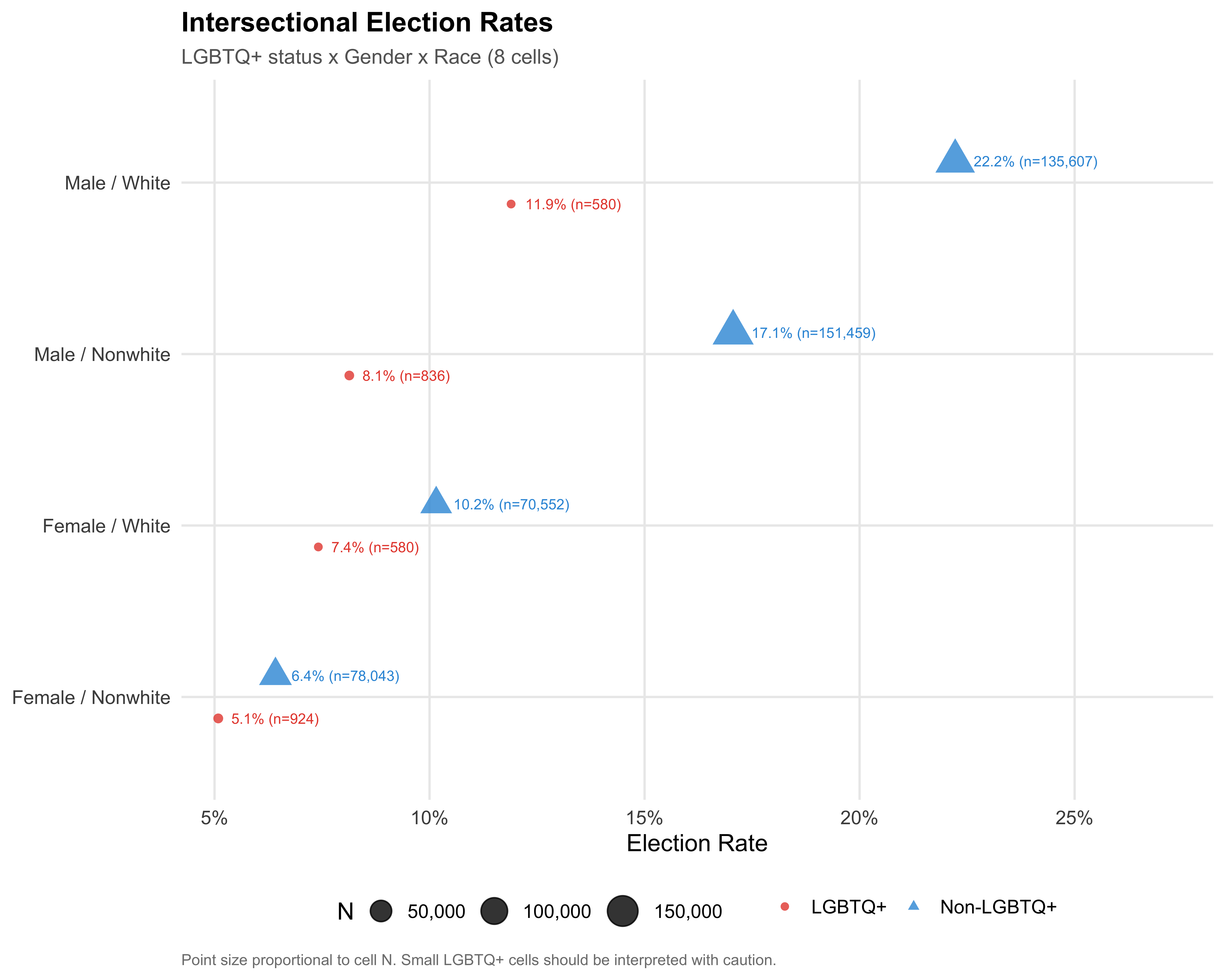
# Triple Intersection: LGBTQ+ x Gender x Race
## Eight-Cell Table
The table below cross-tabulates LGBTQ+ status, gender (Female/Male), and race (White/Nonwhite) to produce eight intersectional cells. For each cell, we report the count, number elected, election rate with 95% confidence intervals, and mean campaign revenue. Cells with fewer than 30 observations are flagged with an asterisk.
::: {.callout-note}
## Pooled Across Positions
The triple intersection analysis pools across city councilors and mayors/vice-mayors. With 8 intersectional cells (2 LGBTQ+ statuses x 2 genders x 2 races), further disaggregation by position would produce 24 cells. Given that the LGBTQ+ executive candidate pool contains only ~91 individuals, many cells would have fewer than 5 observations, rendering statistical comparisons unreliable. Position-specific two-way intersections are available in the tabs above.
:::
```{r tbl-triple}
#| label: tbl-triple
#| tbl-cap: "Triple Intersection: LGBTQ+ Status x Gender x Race"
triple <- df %>%
  filter(!is.na(female), !is.na(nonwhite), !is.na(elected)) %>%
  mutate(
    lgbtq_group  = if_else(lgbtq_candidate, "LGBTQ+", "Non-LGBTQ+"),
    gender_label = if_else(female, "Female", "Male"),
    race_label   = if_else(nonwhite, "Nonwhite", "White")
  ) %>%
  group_by(lgbtq_group, gender_label, race_label) %>%
  summarise(
    N             = n(),
    Elected       = sum(elected),
    `Elect. Rate` = mean(elected),
    `Mean Rev.`   = mean(total_revenue, na.rm = TRUE),
    .groups = "drop"
  ) %>%
  arrange(lgbtq_group, gender_label, race_label) %>%
  rowwise() %>%
  mutate(
    ci = list(binom.test(Elected, N)$conf.int),
    CI_low = ci[1],
    CI_high = ci[2],
    small_n = N < 30
  ) %>%
  ungroup() %>%
  select(-ci)

triple %>%
  mutate(
    `Elect. Rate` = paste0(format_pct(`Elect. Rate`),
                           ifelse(small_n, " *", "")),
    `95% CI` = paste0("[", format_pct(CI_low), ", ", format_pct(CI_high), "]"),
    `Mean Rev.`   = format_brl(`Mean Rev.`)
  ) %>%
  rename(`LGBTQ+ Status` = lgbtq_group, Gender = gender_label, Race = race_label) %>%
  select(-CI_low, -CI_high, -small_n) %>%
  kable(align = c("l", "l", "l", "r", "r", "r", "r", "r"))
```
\* indicates N < 30; interpret with caution.
```{r fig-triple-dot}
#| label: fig-triple-dot
#| fig-cap: "Election Rate by LGBTQ+ Status, Gender, and Race (Dot Plot)"
#| fig-height: 8
triple %>%
  mutate(
    cell_label = paste(gender_label, race_label, sep = " / "),
    rate = `Elect. Rate`
  ) %>%
  ggplot(aes(x = rate, y = reorder(cell_label, rate),
             color = lgbtq_group, shape = lgbtq_group)) +
  geom_point(aes(size = N), alpha = 0.8,
             position = position_dodge(width = 0.5)) +
  geom_text(aes(label = paste0(format_pct(rate), " (n=", format_n(N), ")")),
            position = position_dodge(width = 0.5),
            hjust = -0.15, size = 3, show.legend = FALSE) +
  scale_color_manual(values = pal_lgbtq, name = NULL) +
  scale_shape_manual(values = c("LGBTQ+" = 16, "Non-LGBTQ+" = 17), name = NULL) +
  scale_size_continuous(range = c(2, 8), name = "N", labels = comma) +
  scale_x_continuous(labels = percent, expand = expansion(mult = c(0.05, 0.35))) +
  labs(
    x        = "Election Rate",
    y        = NULL,
    title    = "Intersectional Election Rates",
    subtitle = "LGBTQ+ status x Gender x Race (8 cells)",
    caption  = "Point size proportional to cell N. Small LGBTQ+ cells should be interpreted with caution."
  )

save_figure(last_plot(), "06_triple_dot", height = 8)
```
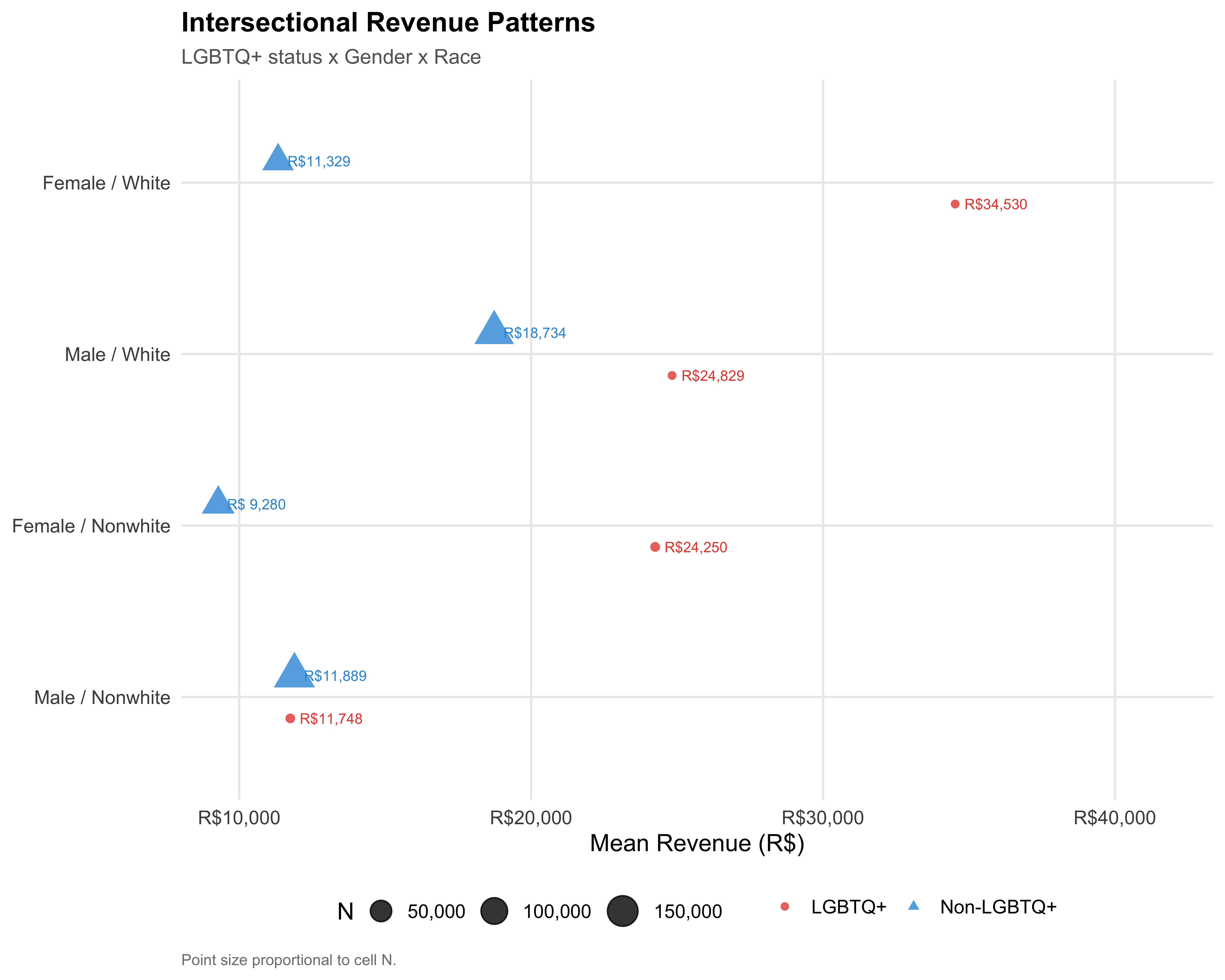
```{r fig-triple-revenue}
#| label: fig-triple-revenue
#| fig-cap: "Mean Revenue by LGBTQ+ Status, Gender, and Race"
#| fig-height: 8
triple %>%
  mutate(cell_label = paste(gender_label, race_label, sep = " / ")) %>%
  ggplot(aes(x = `Mean Rev.`, y = reorder(cell_label, `Mean Rev.`),
             color = lgbtq_group, shape = lgbtq_group)) +
  geom_point(aes(size = N), alpha = 0.8,
             position = position_dodge(width = 0.5)) +
  geom_text(aes(label = format_brl(`Mean Rev.`)),
            position = position_dodge(width = 0.5),
            hjust = -0.15, size = 3, show.legend = FALSE) +
  scale_color_manual(values = pal_lgbtq, name = NULL) +
  scale_shape_manual(values = c("LGBTQ+" = 16, "Non-LGBTQ+" = 17), name = NULL) +
  scale_size_continuous(range = c(2, 8), name = "N", labels = comma) +
  scale_x_continuous(labels = label_dollar(prefix = "R$", big.mark = ","),
                     expand = expansion(mult = c(0.05, 0.35))) +
  labs(
    x        = "Mean Revenue (R$)",
    y        = NULL,
    title    = "Intersectional Revenue Patterns",
    subtitle = "LGBTQ+ status x Gender x Race",
    caption  = "Point size proportional to cell N."
  )

save_figure(last_plot(), "06_triple_revenue", height = 8)
```
::: {.callout-important}
## Compounding Disadvantage
The triple intersection tests whether multiple marginalized identities (LGBTQ+, female, nonwhite) produce compounding disadvantage that is greater than the sum of its parts, or whether the effects are merely additive. The dot plots and table above allow direct comparison of the most and least privileged intersectional cells.
:::
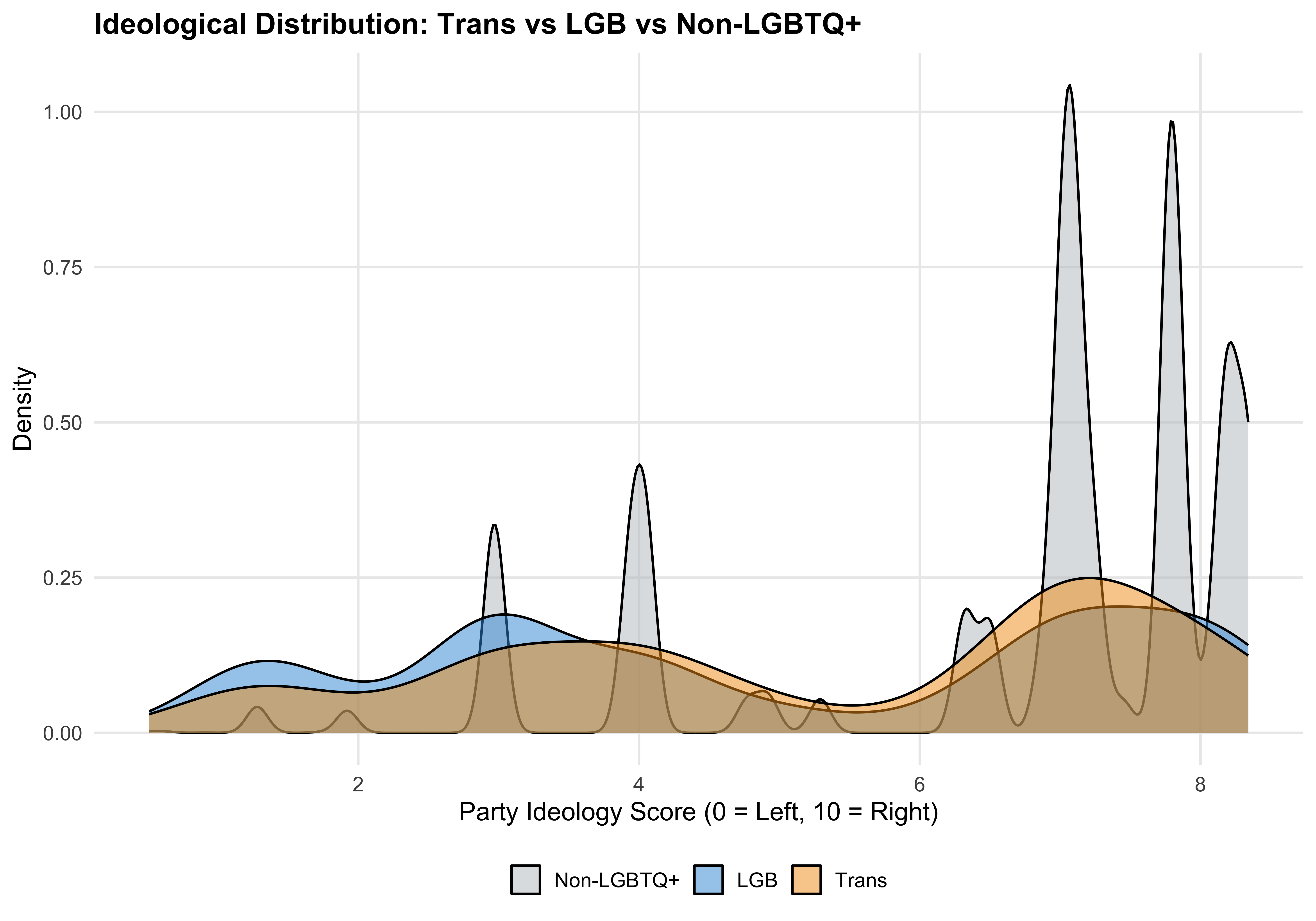
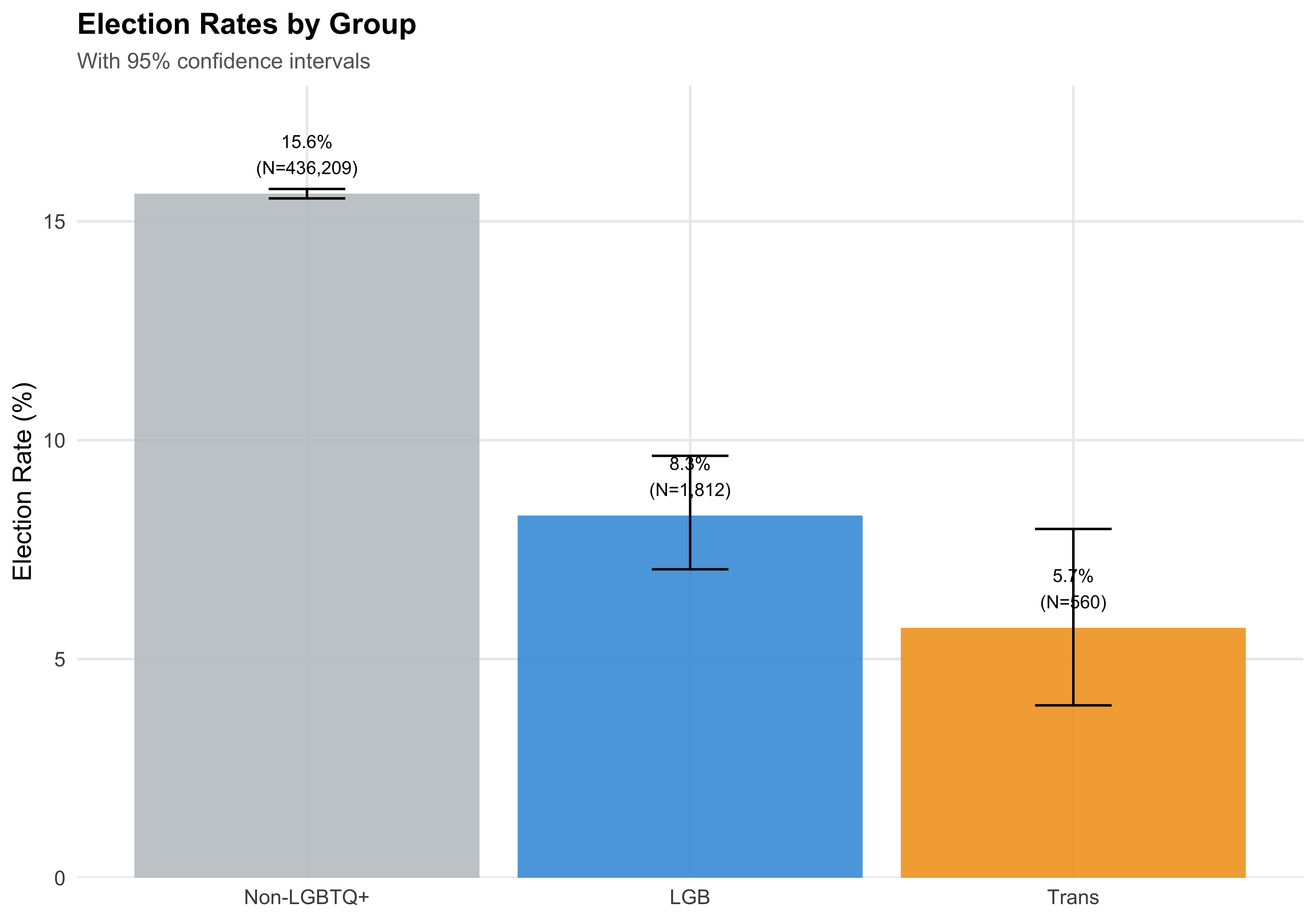
# Trans vs LGB vs Non-LGBTQ+
The analyses above compare LGBTQ+ candidates as a single group against non-LGBTQ+ candidates. But the LGBTQ+ umbrella encompasses distinct experiences: trans candidates face identity-specific barriers (documentation, social stigma) that differ from those faced by cisgender LGB candidates. This section uses a three-way comparison --- Trans, LGB (cisgender), and Non-LGBTQ+ --- to reveal whether the "LGBTQ+ effect" is driven primarily by one subgroup.
::: {.callout-note}
## Pooled Across Positions
This three-way comparison pools across positions because the Trans group contains too few executive candidates (mayors/vice-mayors) to sustain position-specific breakdowns. Among LGBTQ+ executive candidates, the trans subgroup has very small cell sizes that would make separate estimates unreliable.
:::
## Demographic Profile
```{r tbl-threeway-demo}
#| label: tbl-threeway-demo
#| tbl-cap: "Demographic Profile: Trans vs LGB vs Non-LGBTQ+"
threeway_demo <- df %>%
  group_by(threeway_group) %>%
  summarise(
    N = n(),
    `% Female` = round(mean(female, na.rm = TRUE) * 100, 1),
    `% Nonwhite` = round(mean(nonwhite, na.rm = TRUE) * 100, 1),
    `Mean Age` = round(mean(age, na.rm = TRUE), 1),
    `% College+` = round(mean(education_simple == "College+", na.rm = TRUE) * 100, 1),
    `Median Revenue` = format_brl(median(total_revenue, na.rm = TRUE)),
    `Election Rate (%)` = round(mean(elected, na.rm = TRUE) * 100, 1),
    .groups = "drop"
  )

threeway_demo %>%
  rename(Group = threeway_group) %>%
  kable(align = c("l", rep("r", 7)), format.args = list(big.mark = ","))
```
## Ideology Comparison
```{r fig-threeway-ideology}
#| label: fig-threeway-ideology
#| fig-cap: "Ideology Score Distribution: Trans vs LGB vs Non-LGBTQ+"
ggplot(df %>% filter(!is.na(ideology_score)),
       aes(x = ideology_score, fill = threeway_group)) +
  geom_density(alpha = 0.5) +
  scale_fill_manual(values = c("Non-LGBTQ+" = "#BDC3C7", "LGB" = "#3498DB", "Trans" = "#F39C12")) +
  labs(
    x = "Party Ideology Score (0 = Left, 10 = Right)",
    y = "Density",
    fill = NULL,
    title = "Ideological Distribution: Trans vs LGB vs Non-LGBTQ+"
  )

save_figure(last_plot(), "06_threeway_ideology")
```
## Election Rates
```{r fig-threeway-election}
#| label: fig-threeway-election
#| fig-cap: "Election Rates: Trans vs LGB vs Non-LGBTQ+"
threeway_rates <- df %>%
  filter(!is.na(elected)) %>%
  group_by(threeway_group) %>%
  summarise(
    n = n(),
    elected = sum(elected),
    rate = elected / n,
    ci_lo = binom.test(elected, n)$conf.int[1],
    ci_hi = binom.test(elected, n)$conf.int[2],
    .groups = "drop"
  )

ggplot(threeway_rates, aes(x = threeway_group, y = rate * 100,
                            fill = threeway_group)) +
  geom_col(alpha = 0.85) +
  geom_errorbar(aes(ymin = ci_lo * 100, ymax = ci_hi * 100), width = 0.2) +
  geom_text(aes(label = paste0(round(rate * 100, 1), "%\n(N=", format_n(n), ")")),
            vjust = -0.5, size = 3.5) +
  scale_fill_manual(values = c("Non-LGBTQ+" = "#BDC3C7", "LGB" = "#3498DB", "Trans" = "#F39C12"),
                    guide = "none") +
  scale_y_continuous(expand = expansion(mult = c(0, 0.15))) +
  labs(
    x = NULL, y = "Election Rate (%)",
    title = "Election Rates by Group",
    subtitle = "With 95% confidence intervals"
  )

save_figure(last_plot(), "06_threeway_election")
```
## Revenue Comparison
```{r tbl-threeway-revenue}
#| label: tbl-threeway-revenue
#| tbl-cap: "Revenue and Funding Sources: Trans vs LGB vs Non-LGBTQ+"
threeway_rev <- df %>%
  filter(total_revenue > 0) %>%
  group_by(threeway_group) %>%
  summarise(
    N = n(),
    `Median Revenue` = format_brl(median(total_revenue)),
    `Mean Revenue` = format_brl(mean(total_revenue)),
    `% Self-Funded` = round(mean(pct_self, na.rm = TRUE), 1),
    `% Party` = round(mean(pct_party, na.rm = TRUE), 1),
    `% Individual` = round(mean(pct_individual, na.rm = TRUE), 1),
    `Median Donors` = round(median(n_unique_donors, na.rm = TRUE), 1),
    .groups = "drop"
  )

threeway_rev %>%
  rename(Group = threeway_group) %>%
  kable(align = c("l", rep("r", 7)), format.args = list(big.mark = ","))
```
::: {.callout-note}
## Trans vs LGB
The three-way comparison reveals whether the aggregate LGBTQ+ patterns are driven by one subgroup or represent a shared experience. Trans candidates may face distinct barriers --- reflected in different election rates, revenue levels, and funding source composition --- that are masked when the LGBTQ+ category is treated as monolithic.
:::
# Trans-Specific Intersectional Profile
Trans candidates constitute a small but highly visible subgroup. Given the small N, disaggregating trans candidates across multiple dimensions simultaneously yields very small cell sizes. Rather than producing unreliable cross-tabulations, we present a descriptive profile.
## Trans Candidate Demographics
The tables below provide a descriptive profile of trans candidates across key intersectional dimensions: gender and race, education and region, party affiliation, and ideology. Given the small sample size, these should be read as a descriptive inventory rather than as evidence of statistical patterns.
```{r tbl-trans-profile}
#| label: tbl-trans-profile
#| tbl-cap: "Trans Candidates: Intersectional Profile"
trans_profile <- df %>%
  filter(trans_candidate) %>%
  mutate(
    gender_label = if_else(female, "Female", "Male"),
    race_label   = if_else(nonwhite, "Nonwhite", "White"),
    elected_label = if_else(elected, "Elected", "Not elected", missing = "Unknown")
  )

# Summary table by key intersections
trans_cross <- trans_profile %>%
  filter(!is.na(female), !is.na(nonwhite)) %>%
  group_by(gender_label, race_label) %>%
  summarise(
    N            = n(),
    `Mean Age`   = round(mean(age, na.rm = TRUE), 1),
    Elected      = sum(elected, na.rm = TRUE),
    `Mean Rev.`  = format_brl(mean(total_revenue, na.rm = TRUE)),
    .groups = "drop"
  ) %>%
  rename(Gender = gender_label, Race = race_label)

trans_cross %>%
  kable(align = c("l", "l", "r", "r", "r", "r"))
```
```{r tbl-trans-education-region}
#| label: tbl-trans-education-region
#| tbl-cap: "Trans Candidates by Education and Region"
trans_edu_region <- trans_profile %>%
  filter(!is.na(education_simple), !is.na(region)) %>%
  count(education_simple, region) %>%
  pivot_wider(names_from = region, values_from = n, values_fill = 0) %>%
  rename(Education = education_simple)

trans_edu_region %>%
  kable(align = c("l", rep("r", ncol(trans_edu_region) - 1)))
```
```{r tbl-trans-party}
#| label: tbl-trans-party
#| tbl-cap: "Trans Candidates by Party (Top Parties)"
trans_profile %>%
  count(party_abbrev, sort = TRUE) %>%
  head(15) %>%
  left_join(
    trans_profile %>%
      group_by(party_abbrev) %>%
      summarise(
        elected = sum(elected, na.rm = TRUE),
        mean_rev = format_brl(mean(total_revenue, na.rm = TRUE)),
        .groups = "drop"
      ),
    by = "party_abbrev"
  ) %>%
  rename(
    Party     = party_abbrev,
    `N Trans` = n,
    Elected   = elected,
    `Mean Rev.` = mean_rev
  ) %>%
  kable(align = c("l", "r", "r", "r"))
```
```{r tbl-trans-ideology}
#| label: tbl-trans-ideology
#| tbl-cap: "Trans Candidates by Ideology Category"
trans_profile %>%
  filter(!is.na(ideology_category)) %>%
  count(ideology_category) %>%
  mutate(pct = format_pct(n / sum(n))) %>%
  rename(Ideology = ideology_category, N = n, `%` = pct) %>%
  kable(align = c("l", "r", "r"))
```
::: {.callout-warning}
## Small-N Limitations
With `r format_n(sum(df$trans_candidate, na.rm = TRUE))` trans candidates total, intersectional breakdowns produce very small cell sizes. The numbers above should be read as a descriptive inventory, not as evidence of statistical patterns. Any future regression analysis involving trans candidates should consider pooling strategies or Bayesian approaches that handle sparse data appropriately.
:::
## Trans Candidate Enumeration
For maximum transparency with the small trans sample, we list the full distribution across key variable combinations.
```{r tbl-trans-enumeration}
#| label: tbl-trans-enumeration
#| tbl-cap: "Trans Candidates: Full Cross-Tabulation of Key Variables"
trans_enum <- df %>%
  filter(trans_candidate) %>%
  filter(!is.na(female), !is.na(nonwhite), !is.na(education_simple), !is.na(region)) %>%
  count(
    Gender    = if_else(female, "Female", "Male"),
    Race      = if_else(nonwhite, "Nonwhite", "White"),
    Education = education_simple,
    Region    = region,
    name      = "N"
  ) %>%
  arrange(desc(N))

trans_enum %>%
  kable(align = c("l", "l", "l", "l", "r"))
```
# Summary
This intersectional analysis examines the layered nature of political marginalization in Brazil's 2024 municipal elections:
1. **Gender x LGBTQ+**: The interaction between LGBTQ+ status and gender is examined through election rates and campaign revenue, revealing whether the LGBTQ+ gap differs for male and female candidates.
2. **Race x LGBTQ+**: The interaction between LGBTQ+ status and race tests whether nonwhite LGBTQ+ candidates face compounding disadvantage, and whether the effects are additive or multiplicative.
3. **Ideology x LGBTQ+**: The interaction plot reveals the degree to which the partisan environment moderates the relationship between LGBTQ+ status and electoral outcomes across left, center, and right parties.
4. **Triple intersection**: The eight-cell analysis (LGBTQ+ x gender x race) identifies the most and least advantaged candidate profiles, providing a map of intersectional privilege and disadvantage.
5. **Trans specificity**: Trans candidates, despite their small numbers, are an essential part of the story. Their intersectional profiles --- distributed across specific parties, regions, and demographic groups --- warrant dedicated attention in both descriptive and inferential work.
These patterns motivate the regression analysis in subsequent work, where we can test whether the observed intersectional gaps survive controls for municipality size, position type, incumbency, and campaign spending.